本文最后更新于:2025年4月30日 下午
Shapely 是 Python 中一个优秀的平面图形处理库,本文跟读翻译官方文档2.0.4版本的用户手册,解释了如何使用 Shapely Python 软件包进行几何计算。
简介(Introduction)
官方文档:https://shapely.readthedocs.io/en/stable/manual.html#introduction
文中所有介绍以及代码示例均基于 shapely v2.0.4
确定性空间分析是计算方法在农业,生态学,流行病学,社会学和许多其他领域的问题的重要组成部分。这些动物栖息地的调查周长/面积比率是多少?这个小镇的哪些房产与这个新的洪水模型中的50年洪水轮廓线相交?有“ A”和“ B”标记的古代陶器发现点的范围是什么,范围在哪里重叠?从家到办公室,哪条路最能避免垃圾邮件的定位?这些只是几个可以通过非统计空间分析解决的问题,更具体地说,是计算几何。
Shapely 是一个用于集合论分析和平面特性操作的 Python 包,使用的函数来自著名的和广泛部署的 GEOS 库。GEOS 是 Java 拓扑套件(JTS)的一个端口,是 PostGIS 空间扩展的几何引擎,用于 PostgreSQL RDBMS。JTS 和 GEOS 的设计在很大程度上遵循了开放地理空间协会的简单特性访问规范[1] ,而 Shapely 主要遵循同一套标准类和操作。Shapely 因此深深植根于地理信息系统(GIS)世界的惯例,但是渴望对处理非常规问题的程序员同样有用。
Shapely 的第一个前提是 Python 程序员应该能够在 RDBMS 之外执行 PostGIS 类型的几何操作。并非所有地理数据都源自或驻留在 RDBMS 中,或者最好使用 SQL 进行处理。我们可以将数据加载到一个空间 RDBMS 中来完成工作,但是如果没有任务来管理数据库中的数据(“ RDBMS”中的“ M”) ,那么我们就使用了错误的工具来完成这项工作。第二个前提是特征的持久性、序列化和映射投影是重要的,但是是正交的问题。你可能不需要100个 GIS 格式的读者和作者,也不需要大量的国家平面投影,Shapely 也不会给你带来负担。第三个前提是 Python 习惯用法胜过 GIS (在本例中是 Java,因为 GEOS 库源自 Java 项目 JTS)习惯用法。
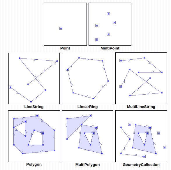
空间数据模型
Shapely 实现的几何对象的基本类型是点、曲线和曲面。每一个都与平面上的三组(可能是无限的)点相关联。一个特征的内部(interior )、边界(boundary )和外部(exterior )集合是相互排斥的,它们的结合与整个平面一致。
类型
内部
边界
外部
拓扑维数
Point
一个点
无
其他所有点
0
Curve
线上所有的点(不包含起点、终点)
起点、终点
其他所有点
1
Surface
边缘内部的所有点
边缘曲线上的所有点
其他所有点
2
点类型由 Point 类实现; 曲线由 LineString 和 LinearRing 类实现; 曲面由 Polygon 类实现。Shapely 不实现平滑曲线(即具有连续的切线)。所有曲线都必须用线性样条逼近。所有的圆形斑块都必须用线性样条曲线所包围的区域来近似。
点的集合由 MultiPoint 类实现,曲线的集合由 MultiLineString 类实现,曲面的集合由 MultiPolygon 类实现。这些集合在计算上并不重要,但是对于建模某些类型的特性非常有用。
几何对象(Geometric Objects)
官方文档:https://shapely.readthedocs.io/en/stable/manual.html#geometric-objects
Point、 LineString 和 LinearRing 的实例最重要的属性是一个有限的坐标序列,它决定了它们的内部、边界和外部点集。线条字符串可以由最少2个点确定,但包含无限多个点。坐标序列是不可变的。在构建实例时可以使用第三个 z 坐标值,但对几何分析没有影响。所有操作都在 x-y 平面中执行。
在所有构造函数中,数值都被转换为 float 类型。换句话说,Point (0.0)和 Point (0.0.0.0)产生几何等效的实例。当构造实例时,Shapely 不检查拓扑的简单性或有效性,因为在大多数情况下,成本是没有保证的。验证工厂很容易通过需要它们的用户使用: attr: is_valid谓词来实现。
Shapely 是一个平面几何库,z (平面上方或下方的高度)在几何分析中被忽略 。对于用户来说,这里有一个潜在的陷阱: 只有 z 值不同的坐标元组彼此之间没有区别,而且它们的应用程序可能导致令人惊讶的无效几何对象。
一般属性
属性
含义
备注
object.area
返回对象的面积(浮点数)。
object.bounds
返回一个(minx,miny,maxx,maxy)元组(float 值) ,该元组围绕对象。
object.length
返回对象的长度(浮点数)。
object.minimum_clearance
返回移动节点以生成无效几何图形的最小距离。
这可以被认为是一个测量的健壮性的几何形状,其中较大的最小间隙值表示一个更健壮的几何形状。如果一个几何图形没有最小间隙,比如一个点,那么这个函数将返回数学无穷大。
object.geom_type
返回指定对象的几何类型的字符串
minimum_clearance 示例
1
2
3
4
5
from shapely import Polygon0 , 0 ], [1 , 0 ], [1 , 1 ], [0 , 1 ], [0 , 0 ]]).minimum_clearance1.0
geom_type 示例s
1
2
3
4
5
from shapely import Point, LineString0 , 0 ).geom_type'Point'
一般方法
属性
含义
备注
object.distance(other)
返回到其他几何对象的最小距离(浮点数)。
object.hausdorff_distance(other)
返回另一个几何对象的豪斯多夫距离(float)。两个几何图形之间的豪斯多夫距离是任何一个几何图形上的一个点与另一个几何图形上的一个点之间的最远距离。
object.representative_point()
返回一个保证位于几何对象内的点。
hausdorff_distance 示例
1
2
3
4
5
6
point = Point(1 , 1 )line = LineString([(2 , 0 ), (2 , 4 ), (3 , 4 )])point .hausdorff_distance(line)3 .605551275463989 point .distance(Point(3 , 4 ))3 .605551275463989
Points
1 class Point (coordinates )
创建实例
1
2
3
from shapely import Point0.0 , 0.0 )0.0 , 0.0 ))
属性展示
1 2 3 4 5 6 7 8 9 10 11 12 13 14 15 16 17 18 19 20 21 0.0 0.0 0.0 , 0.0 , 0.0 , 0.0 )list (point.coords)0.0 , 0.0 )]0.0 0.0
LineStrings
1 class LineString (coordinates )
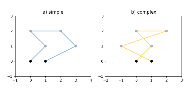
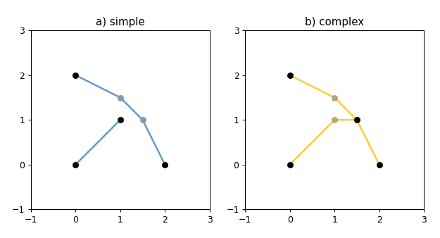
LineString 构造函数接受2个或更多(x,y [ ,z ])点元组的有序序列。
构造的 LineString 对象表示点之间的一个或多个连接的线性样条。在有序的顺序中允许重复的点,但是可能会导致性能损失,应该避免。一个 LineString 可以跨越它自己(也就是说是复杂的而不是简单的)。
示例代码
1
2
3
4
5
6
7
8
9
10
11
12
13
14
15
16
17
18
19
20
21
22
23
24
25
26
27
28
29
30
31
32
33
import matplotlib.pyplot as pltfrom shapely.geometry import LineStringfrom shapely.plotting import plot_line, plot_pointsfrom figures import SIZE, BLACK, BLUE, GRAY, YELLOW, set_limits1 , figsize=SIZE, dpi=90 )121 )0 , 0 ), (1 , 1 ), (0 , 2 ), (2 , 2 ), (3 , 1 ), (1 , 0 )])False , color=BLUE, alpha=0.7 )0.7 )'a) simple' )1 , 4 , -1 , 3 )122 )0 , 0 ), (1 , 1 ), (0 , 2 ), (2 , 2 ), (-1 , 1 ), (1 , 0 )])False , color=YELLOW, alpha=0.7 )0.7 )'b) complex' )2 , 3 , -1 , 3 )
其中 figures.py 需要手动创建 :
后文中的 类似 figures 用法相同,不再赘述
1
2
3
4
5
6
7
8
9
10
11
12
13
14
15
16
17
18
19
20
21
22
23
24
25
26
27
28
29
30
from math import sqrtfrom shapely import affinity5 )-1.0 )/2.0 8.0 '#6699cc' '#999999' '#333333' '#ffcc33' '#339933' '#ff3333' '#000000' def add_origin (ax, geom, origin ):2 )'o' , color=GRAY, zorder=1 )str (xy), xy=xy, ha='center' ,'offset points' , xytext=(0 , 8 ))def set_limits (ax, x0, xN, y0, yN ):range (x0, xN+1 ))range (y0, yN+1 ))"equal" )
属性展示
1
2
3
4
5
6
7
8
9
10
11
12
13
14
15
16
17
18
19
20
21
22
23
24
25
26
27
28
29
30
31
32
from shapely import LineString0 , 0 ), (1 , 1 )])0.0 1.4142135623730951 0.0 , 0.0 , 1.0 , 1.0 )len (line.coords)2 list (line.coords)0.0 , 0.0 ), (1.0 , 1.0 )]0.0 , 0.0 ), (1.0 , 1.0 )]1 :]1.0 , 1.0 )]0 0 , 1 1 )>0.0 , 1.0 ), (2.0 , 3.0 ), Point(4.0 , 5.0 )])0 1 , 2 3 , 4 5 )>
LinearRings
1 class LinearRing (coordinates )
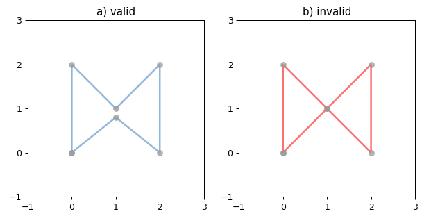
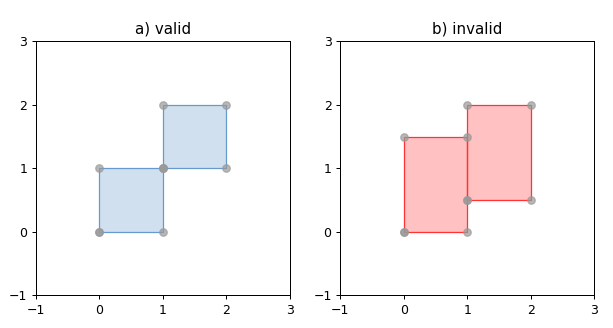
LinearRing 构造函数接受(x,y [ ,z ])点元组的有序序列。
序列可以通过在第一个和最后一个索引中传递相同的值来显式关闭。否则,通过将第一个元组复制到最后一个索引,序列将隐式关闭。与使用 LineString 一样,允许顺序序列中的重复点,但是可能会导致性能损失,因此应该避免。一个线性环不可以跨越自己,也不可以触及自己在一个单一的点。
与 LineStrings 不同的就是 Rings 闭环
示例代码
1
2
3
4
5
6
7
8
9
10
11
12
13
14
15
16
17
18
19
20
21
22
23
24
25
26
27
28
29
30
31
import matplotlib.pyplot as pltfrom shapely.geometry import LinearRingfrom shapely.plotting import plot_line, plot_pointsfrom figures import SIZE, BLUE, GRAY, RED, set_limits1 , figsize=SIZE, dpi=90 )121 )0 , 0 ), (0 , 2 ), (1 , 1 ), (2 , 2 ), (2 , 0 ), (1 , 0.8 ), (0 , 0 )])False , color=BLUE, alpha=0.7 )0.7 )'a) valid' )1 , 3 , -1 , 3 )122 )0 , 0 ), (0 , 2 ), (1 , 1 ), (2 , 2 ), (2 , 0 ), (1 , 1 ), (0 , 0 )])False , color=RED, alpha=0.7 )0.7 )'b) invalid' )1 , 3 , -1 , 3 )
运行效果
Shapely 不会阻止出问题的环的产生,但是当它们被操作时会产生错误。
属性展示
和 LineStrings 很像
1
2
3
4
5
6
7
8
9
10
11
12
13
14
15
16
17
18
19
20
21
22
23
24
from shapely import LinearRing0 , 0 ), (1 , 1 ), (1 , 0 )])0.0 3.414213562373095 0.0 , 0.0 , 1.0 , 1.0 )len (ring.coords)4 list (ring.coords)0.0 , 0.0 ), (1.0 , 1.0 ), (1.0 , 0.0 ), (0.0 , 0.0 )]0 0 , 1 1 , 1 0 , 0 0 )>
Polygons
1 class Polygon (shell [, holes =None ])
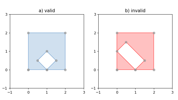
多边形构造函数有两个位置参数。第一个是(x,y [ ,z ])点元组的有序序列,它被完全按照 LinearRing 的情况处理。第二个是一个可选的环状序列的无序序列,指定特征的内部边界或“孔”。
一个有效的多边形的环不能相互交叉,但只能在一个点接触。同样,Shapely 不会阻止无效特性的创建,但在操作它们时会引发异常。
示例代码 1
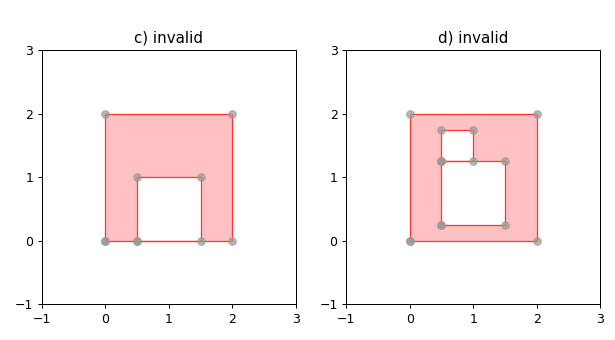
1
2
3
4
5
6
7
8
9
10
11
12
13
14
15
16
17
18
19
20
21
22
23
24
25
26
27
28
29
30
31
32
33
34
35
36
import matplotlib.pyplot as pltfrom shapely.geometry import Polygonfrom shapely.plotting import plot_polygon, plot_pointsfrom figures import SIZE, BLUE, GRAY, RED, set_limits1 , figsize=SIZE, dpi=90 )121 )0 , 0 ), (0 , 2 ), (2 , 2 ), (2 , 0 ), (0 , 0 )]int = [(1 , 0 ), (0.5 , 0.5 ), (1 , 1 ), (1.5 , 0.5 ), (1 , 0 )][::-1 ]int ])False , color=BLUE)0.7 )'a) valid' )1 , 3 , -1 , 3 )122 )0 , 0 ), (0 , 2 ), (2 , 2 ), (2 , 0 ), (0 , 0 )]int = [(1 , 0 ), (0 , 1 ), (0.5 , 1.5 ), (1.5 , 0.5 ), (1 , 0 )][::-1 ]int ])False , color=RED)0.7 )'b) invalid' )1 , 3 , -1 , 3 )
运行效果
示例代码 2
1
2
3
4
5
6
7
8
9
10
11
12
13
14
15
16
17
18
19
20
21
22
23
24
25
26
27
28
29
30
31
32
33
34
35
36
37
import matplotlib.pyplot as pltfrom shapely.geometry import Polygonfrom shapely.plotting import plot_polygon, plot_pointsfrom figures import GRAY, RED, SIZE, set_limits1 , figsize=SIZE, dpi=90 )121 )0 , 0 ), (0 , 2 ), (2 , 2 ), (2 , 0 ), (0 , 0 )]int = [(0.5 , 0 ), (1.5 , 0 ), (1.5 , 1 ), (0.5 , 1 ), (0.5 , 0 )]int ])False , color=RED)0.7 )'c) invalid' )1 , 3 , -1 , 3 )122 )0 , 0 ), (0 , 2 ), (2 , 2 ), (2 , 0 ), (0 , 0 )]0.5 , 0.25 ), (1.5 , 0.25 ), (1.5 , 1.25 ), (0.5 , 1.25 ), (0.5 , 0.25 )]0.5 , 1.25 ), (1 , 1.25 ), (1 , 1.75 ), (0.5 , 1.75 )]False , color=RED)0.7 )'d) invalid' )1 , 3 , -1 , 3 )
运行效果
上述代码运行结果中,仅蓝色块为合法多边形,其余由于多点重合、边重合为非法多边形。
属性展示
1
2
3
4
5
6
7
8
9
10
11
12
13
14
15
16
17
18
19
20
21
22
23
24
25
26
27
28
29
30
31
32
33
from shapely import Polygon0 , 0 ), (1 , 1 ), (1 , 0 )])0.5 3.414213562373095 0.0 , 0.0 , 1.0 , 1.0 )list (polygon.exterior.coords)0.0 , 0.0 ), (1.0 , 1.0 ), (1.0 , 0.0 ), (0.0 , 0.0 )]list (polygon.interiors)0 , 0 ), (1 , 1 ), (1 , 0 )]0.5 1.0 ).exterior, [r])6.5507620529190325
box 矩形多边形经常出现,可以方便地使用 shapely.geomey.box ()函数构造。
1 shapely.geometry.box(minx, miny, maxx, maxy, ccw =True )
示例代码
1
2
3
4
5
6
from shapely import box0.0 , 0.0 , 1.0 , 1.0 )1 0 , 1 1 , 0 1 , 0 0 , 1 0 ))>list (b.exterior.coords)1.0 , 0.0 ), (1.0 , 1.0 ), (0.0 , 1.0 ), (0.0 , 0.0 ), (1.0 , 0.0 )]
orient 要获得具有已知方向的多边形,请使用 shapely.geomey.polygon.orient () :
1 shapely.geometry .polygon .orient(polygon , sign=1.0 )
返回给定多边形的一个正确定向的副本。结果的签名区域将具有给定的符号。1.0的符号意味着产品外环的坐标将逆时针方向和内环(孔)将顺时针方向。
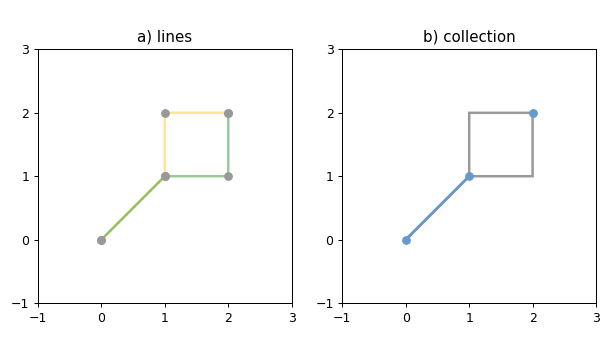
Collections
几何对象的异构集合可能来自某些 Shapely 操作。例如,两个 LineString 可能在一条线上和一个点上相交。为了表示这类结果,Shapely 提供了类似于冻结集的、不可变的几何对象集合。集合可以是同构的(MultiPoint 等)或异构的。
1
2
3
4
5
6
7
8
9
a = LineString([(0 , 0 ), (1 , 1 ), (1 ,2 ), (2 ,2 )])0 , 0 ), (1 , 1 ), (2 ,1 ), (2 ,2 )])0 0 , 1 1 ), POINT (2 2 ))>list (x.geoms)0 0 , 1 1 )>, <POINT (2 2 )>]
示例代码
1
2
3
4
5
6
7
8
9
10
11
12
13
14
15
16
17
18
19
20
21
22
23
24
25
26
27
28
29
30
31
32
33
34
35
36
37
38
39
import matplotlib.pyplot as pltfrom shapely.geometry import LineStringfrom shapely.plotting import plot_line, plot_pointsfrom figures import BLUE, GRAY, YELLOW, GREEN, SIZE, set_limits1 , figsize=SIZE, dpi=90 )0 , 0 ), (1 , 1 ), (1 ,2 ), (2 ,2 )])0 , 0 ), (1 , 1 ), (2 ,1 ), (2 ,2 )])121 )False , color=YELLOW, alpha=0.5 )False , color=GREEN, alpha=0.5 )'a) lines' )1 , 3 , -1 , 3 )122 )False )False )0 ], ax=ax, color=BLUE)1 ], ax=ax, color=BLUE)'b) collection' )1 , 3 , -1 , 3 )
运行效果
一条绿色和一条黄色的线,它们沿着一条直线在一个点相交; b)交点(蓝色)是一个包含一个 LineString 和一个 Point 的集合。
Collections of Points
MultiPoint 构造函数接受(x,y [ ,z ])点元组序列。
1 class MultiPoint (points )
属性展示
1
2
3
4
5
6
7
8
9
10
11
12
13
14
15
16
17
18
19
20
from shapely import MultiPoint0.0 , 0.0 ), (1.0 , 1.0 )])0.0 0.0 0.0 , 0.0 , 1.0 , 1.0 )list (points.geoms)0 0 )>, <POINT (1 1 )>]0 , 0 ), Point(1 , 1 )])0 0 , 1 1 )>
Collections of Lines
MultiLineString 构造函数接受一系列类似行的序列或对象。
1 class MultiLineString (lines )
示例代码
1
2
3
4
5
6
7
8
9
10
11
12
13
14
15
16
17
18
19
20
21
22
23
24
25
26
27
28
29
30
31
32
33
34
35
36
import matplotlib.pyplot as pltfrom shapely.geometry import MultiLineStringfrom shapely.plotting import plot_line, plot_pointsfrom figures import SIZE, BLACK, BLUE, GRAY, YELLOW, set_limits1 , figsize=SIZE, dpi=90 )121 )0 , 0 ), (1 , 1 )), ((0 , 2 ), (1 , 1.5 ), (1.5 , 1 ), (2 , 0 ))])0.7 )'a) simple' )1 , 3 , -1 , 3 )122 )0 , 0 ), (1 , 1 ), (1.5 , 1 )), ((0 , 2 ), (1 , 1.5 ), (1.5 , 1 ), (2 , 0 ))])0.7 )'b) complex' )1 , 3 , -1 , 3 )
属性展示
1
2
3
4
5
6
7
8
9
10
11
12
13
14
15
16
17
18
19
20
21
22
23
24
25
26
27
from shapely import MultiLineString0 , 0 ), (1 , 1 )), ((-1 , 0 ), (1 , 0 ))]0.0 3.414213562373095 1.0 , 0.0 , 1.0 , 1.0 )len (lines.geoms)2 print (list (lines.geoms))0 0 , 1 1 )>, <LINESTRING (-1 0 , 1 0 )>]0 0 , 1 1 ), (-1 0 , 1 0 ))>0 0 , 1 1 ), (-1 0 , 1 0 ))>
Collections of Polygons
MultiPolygon 构造函数接受一个外环和空穴列表元组序列: [((a1,… ,aM) ,[(b1,… ,bN) ,… ]) ,… ]。
1 class MultiPolygon (polygons )
示例代码
1
2
3
4
5
6
7
8
9
10
11
12
13
14
15
16
17
18
19
20
21
22
23
24
25
26
27
28
29
30
31
32
33
34
35
36
37
38
39
import matplotlib.pyplot as pltfrom shapely.geometry import MultiPolygonfrom shapely.plotting import plot_polygon, plot_pointsfrom figures import SIZE, BLUE, GRAY, RED, set_limits1 , figsize=SIZE, dpi=90 )121 )0 , 0 ), (0 , 1 ), (1 , 1 ), (1 , 0 ), (0 , 0 )]1 , 1 ), (1 , 2 ), (2 , 2 ), (2 , 1 ), (1 , 1 )]False , color=BLUE)0.7 )'a) valid' )1 , 3 , -1 , 3 )122 )0 , 0 ), (0 , 1.5 ), (1 , 1.5 ), (1 , 0 ), (0 , 0 )]1 , 0.5 ), (1 , 2 ), (2 , 2 ), (2 , 0.5 ), (1 , 0.5 )]False , color=RED)0.7 )'b) invalid' )1 , 3 , -1 , 3 )
运行效果
左边是一个有2个成员的有效多边形,右边是一个无效的多边形,因为它的成员在无限多个点(沿着一条线)接触。
Empty
一个 Empty 特性是一个与空集重合的点集; 不是 None,而是与 set ([]) 类似。可以通过调用不带参数的各种构造函数来创建空特性。空特性几乎不支持任何操作。
1
2
3
4
5
6
7
8
9
line = LineString()True 0.0 list (line.coords)
Coordinate sequences
描述几何图形的坐标列表表示为坐标序列对象。这些序列不应该被直接初始化,而是可以从现有的几何图形中访问,作为几何图形的属性。
可以对坐标序列进行索引、切片和迭代,就好像它们是一个坐标元组列表一样。
1 2 3 4 5 6 7 8 9 10 line.coords[0 ]0.0 , 1.0 )1 :]2.0 , 3.0 ), (4.0 , 5.0 )]for x, y in line.coords:print ("x={}, y={}" .format (x, y))0.0 , y=1.0 2.0 , y=3.0 4.0 , y=5.0
Polygons 的外部和每个内部环都有一个坐标序列。
1
2
3
poly = Polygon([(0 , 0 ), (0 , 1 ), (1 , 1 ), (0 , 0 )])object at ...>
Linear Referencing Methods
使用一维参考系统沿线性特征(如 LineStrings 和 MultiLineStrings)指定位置是有用的。Shapely 支持基于长度或距离的线性引用,评估沿着一个几何物体到一个给定点的投影的距离,或者沿着该物体的一个给定距离的点的距离。
interpolate
沿线性几何物体返回指定距离处的点。
如果归一化参数为 True,则距离将被解释为几何对象长度的一小部分。
1 object .interpolate (distance[, normalized=False] )
就是返回从几何体边缘从起点出发走过一段距离(可以是绝对距离或者是总长度的百分比)之后停在哪里的坐标。
1 2 3 4 5 6 7 8 0 , 0 ), (0 , 1 ), (1 , 1 )]).interpolate(1.5 )0.5 1 )>0 , 0 ), (0 , 1 ), (1 , 1 )]).interpolate(0.75 , normalized=True )0.5 1 )>
project
返回沿着这个几何对象到离另一个对象最近的点的距离。
如果规范化参数为 True,则返回规范化为对象长度的距离。project ()方法是 interpolate() 的逆方法。
1 object .project (other[, normalized=False] )
1 2 3 4 LineString([(0 , 0 ), (0 , 1 ), (1 , 1 )]).project(ip)1.5 0 , 0 ), (0 , 1 ), (1 , 1 )]).project(ip, normalized=True )0.75
谓词和关系(Predicates and Relationships)
几何对象中解释的类型的对象提供标准的谓词作为属性(对于一元谓词)和方法(对于二元谓词)。无论是一进制还是二进制,都返回 True 或 False。
一元谓词(Unary Predicates)
标准一元谓词实现为只读属性属性,都是形状对象的属性。
has_z 如果特性不仅有 x 和 y,而且还有3D (或所谓的2.5 D)几何图形的 z 坐标,则返回 True。
1 2 3 4 Point(0 , 0 ).has_zFalse 0 , 0 , 0 ).has_zTrue
is_ccw 如果坐标为逆时针顺序,则返回 True (用正符号区域包围区域)。此方法仅适用于 LinearRing 对象 。
1 2 LinearRing([(1 ,0 ), (1 ,1 ), (0 ,0 )]).is_ccwTrue
is_empty 如果特性的内部和边界(在点集术语中)与空集重合,则返回 True。
1
2
3
4
Point () .is_empty Point (0 , 0 ) .is_empty
is_ring 如果该特性是一个闭合且简单的 LineString,则返回 True。
1 2 3 4 LineString([(0 , 0 ), (1 , 1 ), (1 , -1 )]).is_ringFalse 0 , 0 ), (1 , 1 ), (1 , -1 )]).is_ringTrue
此属性适用于 LineString 和 LinearRing 实例,但对其他实例没有意义。
is_simple 如果特性没有交叉,则返回 True。
1 2 LineString([(0 , 0 ), (1 , 1 ), (1 , -1 ), (0 , 1 )]).is_simpleFalse
只对 LineStrings 和 LinearRings 有意义。
is_valid 如果一个特性是“有效的”,返回 True.
有效性测试仅对多边形和多边形有意义。对于其他类型的几何图形,总是返回 True。
一个有效的多边形不能有任何重叠的外部或内部环。一个有效的MultiPolygon不能收集任何重叠的多边形。对无效特性的操作可能会失败。
1 2 MultiPolygon([Point(0 , 0 ).buffer(2.0 ), Point(1 , 1 ).buffer(2.0 )]).is_validFalse
is_valid 谓词可用于编写验证修饰符,以确保只有有效的对象从构造函数返回。
1
2
3
4
5
6
7
8
9
10
from functools import wrapsdef validate (func ): @wraps(func ) def wrapper (*args, **kwargs ):if not ob.is_valid:raise TopologicalError("Given arguments do not determine a valid geometric object" )return obreturn wrapper
二元谓词(Binary Predicates)
标准二元谓词作为方法实现。这些谓词评估拓扑、集合论关系。在某些情况下,结果可能不是人们从不同假设开始所期望的那样。所有这些都以另一个几何对象作为参数并返回 True 或 False。
__eq__如果两个对象具有相同的几何类型,并且两个对象的坐标精确匹配,则返回 True。
equals 如果对象的集合论边界、内部和外部与另一个对象的边界、内部和外部重合,则返回 True。
传递给对象构造函数的坐标是这些集合的坐标,并确定它们,但不是集合的整体。对于新用户来说,这是一个潜在的“陷阱”。例如,可以以不同的方式构建等效线。
1
2
3
4
5
6
7
8
9
10
11
a = LineString([(0 , 0 ), (1 , 1 )])0 , 0 ), (0.5 , 0.5 ), (1 , 1 )])0 , 0 ), (0 , 0 ), (1 , 1 )])True False True False
也就是说 __eq__ 表示完全相同 ,equals 表示等效
contains 如果 other 的点均不位于对象的外部且 other 的内部至少有一个点位于对象的内部,则返回 True。
该谓词适用于所有类型,并且与 inside() 相反。表达式 a.contains(b) == b.within(a) 的计算结果始终为 True。
1
2
3
4
5
coords = [(0 , 0 ), (1 , 1 )]0.5 , 0.5 ))True 0.5 , 0.5 ).within(LineString(coords))True
线的端点是其边界的一部分,因此不包含在内。
1 2 LineString(coords).contains(Point(1.0 , 1.0 ))False
二元谓词可以直接用作 filter() 或 itertools.ifilter() 的谓词。
1
2
3
4
5
6
line = LineString(coords)list (filter (line.contains, [Point(), Point(0.5 , 0.5 )]))len (contained)1 0.5 0.5 )>]
covers 如果 other 的每个点都是对象内部或边界上的点,则返回 True。这与 object.contains(other) 类似,只不过它不要求 other 的任何内部点位于 object 的内部。
也就是带着边界。
covered_by 1 object .covered_ by (other)
如果对象的每个点都是其他点的内部或边界上的点,则返回 True。这相当于 other.covers(object)。
covers 的反函数
crosses 如果对象的内部与另一个对象的内部相交但不包含它,并且相交的尺寸小于其中一个或另一个的尺寸,则返回 True。
disjoint 如果对象的边界和内部与另一个对象根本不相交,则返回 True。
intersects 1 object .intersects (other)
如果对象的边界或内部以任何方式与另一个对象的边界或内部相交,则返回 True。
换句话说,如果几何对象有任何共同的边界或内点,则它们相交。
overlaps 如果几何图形具有多个但不是所有的公共点、具有相同的维度,并且几何图形内部的交集具有与几何图形本身相同的维度,则返回 True。
touches 如果对象至少有一个共同点并且其内部不与另一个对象的任何部分相交,则返回 True。
边界相切/相交
1
2
3
4
a = LineString([(0 , 0 ), (1 , 1 )])1 , 1 ), (2 , 2 )])True
within 如果对象的边界和内部仅与另一个对象的内部(而不是其边界或外部)相交,则返回 True。
DE-9IM Relationships
relate
relate() 方法测试对象之间的所有 DE-9IM 关系,上述命名关系谓词是其中的一个子集。
返回一个对象的内部、边界、外部与另一个几何对象的内部、边界、外部之间关系的 DE-9IM 矩阵的字符串表示形式。
1 2 3 4 Point(0 , 0 ).relate(Point(1 , 1 ))'FF0FFF0F2' 0 , 0 ).relate(LineString([(0 , 0 ), (1 , 1 )]))'F0FFFF102'
relate_pattern 1 object .relate_pattern (other, pattern)
如果几何图形之间关系的 DE-9IM 字符串代码满足模式要求,则返回 True,否则返回 False。
relate_pattern() 将两个几何图形的 DE-9IM 代码字符串与指定的模式进行比较。如果字符串与模式匹配,则返回 True,否则返回 False。
指定的模式可以是精确匹配(0、1 或 2)、布尔匹配(T 或 F)或通配符 (*)。例如,"在…内 "谓词的模式是 T*****FF*。
1
2
3
4
5
6
point = Point(0.5 , 0.5 )0 , 0 ), (0 , 1 ), (1 , 1 ), (1 , 0 )])'T*****FF*' )True True
请注意,几何图形的顺序很重要,如下面代码所示。在这个例子中,正方形包含点,但点不包含正方形。
1 2 3 4 point.relate(square)'0FFFFF212' '0F2FF1FF2'
空间分析方法 (Spatial Analysis Methods)
除了布尔属性和方法之外,Shapely 还提供返回新几何对象的分析方法。
集合论方法 (Set-theoretic Methods)
几乎每一个二元谓词方法都有一个对应的方法来返回一个新的几何对象。此外,对象的集合论边界可作为只读属性使用。
这些方法将始终返回一个几何对象。例如,不相交几何体的交集将返回一个空的几何体集合,而不是 None 或 False。要测试结果是否为空,请使用几何体的 is_empty 属性。
boundary
返回代表对象集合论边界的低维对象。
多边形的边界是一条线,线的边界是点的集合。点的边界是一个空集合。
1
2
3
4
5
6
7
8
coords = [((0 , 0 ), (1 , 1 )), ((-1 , 0 ), (1 , 0 ))]1 0 , 0 0 , 1 0 , 1 1 )>list (lines.boundary.geoms)1 0 )>, <POINT (0 0 )>, <POINT (1 0 )>, <POINT (1 1 )>]
centroid 返回对象几何中心点(点)的表示。
1
2
LineString ([(0 , 0 ), (1 , 1 )]).centroid<POINT (0.5 0.5)>
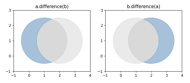
difference 1 object .difference (other)
返回构成此几何对象但不构成其他对象的点的表示。
示例代码
1
2
3
4
5
6
7
8
9
10
11
12
13
14
15
16
17
18
19
20
21
22
23
24
25
26
27
28
29
30
31
32
33
34
35
36
37
38
import matplotlib.pyplot as pltfrom shapely.geometry import Pointfrom shapely.plotting import plot_polygonfrom figures import SIZE, BLUE, GRAY, set_limits1 , figsize=SIZE, dpi=90 )1 , 1 ).buffer(1.5 )2 , 1 ).buffer(1.5 )121 )False , color=GRAY, alpha=0.2 )False , color=GRAY, alpha=0.2 )False , color=BLUE, alpha=0.5 )'a.difference(b)' )1 , 4 , -1 , 3 )122 )False , color=GRAY, alpha=0.2 )False , color=GRAY, alpha=0.2 )False , color=BLUE, alpha=0.5 )'b.difference(a)' )1 , 4 , -1 , 3 )
两个近似圆形的多边形之间的差异。
Shapely 无法将对象与低维对象之间的差异(例如多边形与线或点之间的差异)表示为单个对象,在这些情况下,difference 方法返回名为 self 的对象的副本。
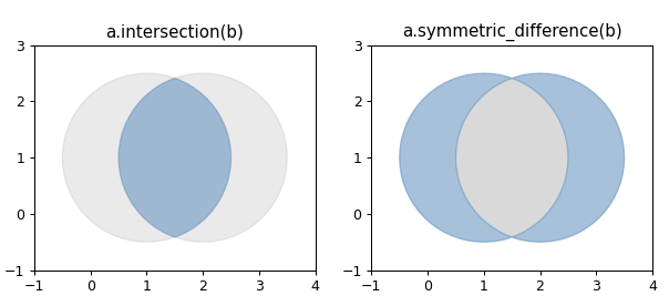
intersection 1 object .intersection (other)
返回此对象与其他几何对象的交集的表示。
1
2
3
4
a = Point(1 , 1 ).buffer(1.5 )2 , 1 ).buffer(1.5 )2.493 0.853 , 2.471 0.707 , 2.435 0.565 , 2.386 0.426 , 2.323 0.293 , ...>
symmetric_difference 1 object .symmetric_difference (other)
返回该对象中不属于其他几何对象中的点以及其他不属于该几何对象中的点的表示。
示例代码
1
2
3
4
5
6
7
8
9
10
11
12
13
14
15
16
17
18
19
20
21
22
23
24
25
26
27
28
29
30
31
32
33
34
35
36
37
38
import matplotlib.pyplot as pltfrom shapely.geometry import Pointfrom shapely.plotting import plot_polygonfrom figures import SIZE, BLUE, GRAY, set_limits1 , figsize=SIZE, dpi=90 )1 , 1 ).buffer(1.5 )2 , 1 ).buffer(1.5 )121 )False , color=GRAY, alpha=0.2 )False , color=GRAY, alpha=0.2 )False , color=BLUE, alpha=0.5 )'a.intersection(b)' )1 , 4 , -1 , 3 )122 )False , color=GRAY, alpha=0.2 )False , color=GRAY, alpha=0.2 )False , color=BLUE, alpha=0.5 )'a.symmetric_difference(b)' )1 , 4 , -1 , 3 )
union 返回此对象和另一个几何对象的点并集的表示。
示例代码
1
2
3
4
5
6
7
8
9
10
11
12
13
14
15
16
17
18
19
20
21
22
23
24
25
26
27
28
29
30
31
32
33
34
35
36
37
38
import matplotlib.pyplot as pltfrom shapely.geometry import Pointfrom shapely.plotting import plot_polygon, plot_linefrom figures import SIZE, BLUE, GRAY, set_limits1 , figsize=SIZE, dpi=90 )1 , 1 ).buffer(1.5 )2 , 1 ).buffer(1.5 )121 )False , color=GRAY, alpha=0.2 )False , color=GRAY, alpha=0.2 )False , color=BLUE, alpha=0.5 )'a.union(b)' )1 , 4 , -1 , 3 )122 )False , color=GRAY, linewidth=3 )False , color=GRAY, linewidth=3 )False , color=BLUE, linewidth=3 )'a.boundary.union(b.boundary)' )1 , 4 , -1 , 3 )
union() 是一种查找多个对象的累积并集的昂贵方法。请参阅 shapely.unary_union() 了解更有效的方法。
重载运算符
其中一些集合论方法可以使用重载运算符来调用:
方法
逻辑运算
运算符
intersection and
&
union or
|
difference minus
-
symmetric_difference xor
^
1
2
3
4
5
6
7
8
9
10
11
from shapely import wkt'POLYGON((0 0, 1 0, 1 1, 0 1, 0 0))' )'POLYGON((0.5 0, 1.5 0, 1.5 1, 0.5 1, 0.5 0))' )0.5 0 , 0.5 1 , 1 1 , 1 0 , 0.5 0 ))>0 0 , 0 1 , 0.5 1 , 1 1 , 1.5 1 , 1.5 0 , 1 0 , 0.5 0 , 0 0 ))>0 0 , 0 1 , 0.5 1 , 0.5 0 , 0 0 ))>'MULTIPOLYGON (((0 0, 0 1, 0.5 1, 0.5 0, 0 0)), ((1 1, 1.5 1, 1.5 0, 1 0, 1 1)))'
构造方法 (Constructive Methods)
有形状的几何对象有几种方法可以产生新的对象,而不是通过集合论分析得出的。
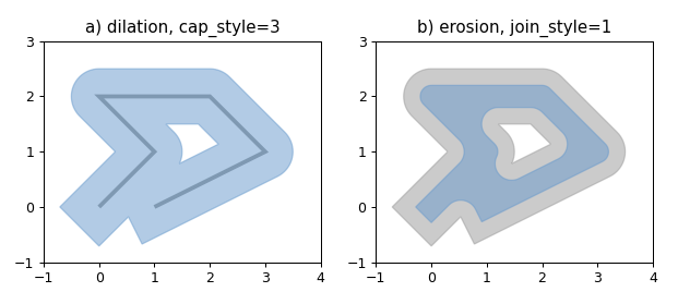
buffer 1 object.buffer(distance, quad_segs =16, cap_style =1, join_style =1, mitre_limit =5.0, single_sided =False )
返回该几何对象给定距离内所有点的近似表示。
cap_style caps 的样式由整数值指定:1(圆形)、2(扁平)、3(方形)。这些值也由对象 shapely.BufferCapStyle 枚举。
shapely.BufferCapStyle
属性
值
round
1
flat
2
square
3
JoinStyle
shapely.BufferJoinStyle
偏移线段之间的连接样式由整数值指定:1(圆形)、2(斜接)和 3(斜角)。这些值也由对象 shapely.BufferJoinStyle 枚举。
属性
值
round
1
mitre
2
bevel
3
正距离具有膨胀效果;负距离,侵蚀。可选的 quad_segs 参数确定用于围绕点近似四分之一圆的线段数。
1
2
3
ine = LineString([(0 , 0 ), (1 , 1 ), (0 , 2 ), (2 , 2 ), (3 , 1 ), (1 , 0 )])dilated = line.buffer(0 .5 )eroded = dilated.buffer(-0 .3 )
示例代码:
1
2
3
4
5
6
7
8
9
10
11
12
13
14
15
16
17
18
19
20
21
22
23
24
25
26
27
28
29
30
31
32
33
34
35
import matplotlib.pyplot as pltfrom shapely.geometry import LineStringfrom shapely.plotting import plot_polygon, plot_linefrom figures import SIZE, BLUE, GRAY, set_limits0 , 0 ), (1 , 1 ), (0 , 2 ), (2 , 2 ), (3 , 1 ), (1 , 0 )])1 , figsize=SIZE, dpi=90 )121 )False , color=GRAY, linewidth=3 )0.5 , cap_style=3 )False , color=BLUE, alpha=0.5 )'a) dilation, cap_style=3' )1 , 4 , -1 , 3 )122 )False , color=GRAY, alpha=0.5 )0.3 )False , color=BLUE, alpha=0.5 )'b) erosion, join_style=1' )1 , 4 , -1 , 3 )
线的膨胀(左)和多边形的腐蚀(右)。新对象显示为蓝色。
quad_segs
点的默认缓冲区(quad_segs 为 16)是一个多边形面,其面积占其近似圆盘面积的 99.8%。
1
2
3
4
5
p = Point(0 , 0 ).buffer(10.0 )len (p.exterior.coords)65 313.6548490545941
当quad_segs为1时,缓冲区是一个方形。
1
2
3
4
5
q = Point(0 , 0 ).buffer(10.0 , 1 )len (q.exterior.coords)5 200.0
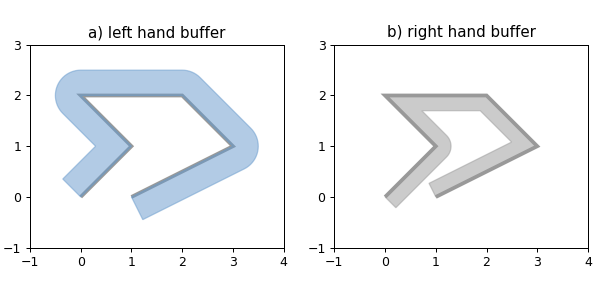
single_side
您可能只需要一侧有一个缓冲区。您可以使用 single_side 选项来实现此效果。
使用的边由缓冲区距离的符号确定:
示例代码
1
2
3
4
5
6
7
8
9
10
11
12
13
14
15
16
17
18
19
20
21
22
23
24
25
26
27
28
29
30
31
32
33
34
35
import matplotlib.pyplot as pltfrom shapely.geometry import LineStringfrom shapely.plotting import plot_polygon, plot_linefrom figures import SIZE, BLUE, GRAY, set_limits0 , 0 ), (1 , 1 ), (0 , 2 ), (2 , 2 ), (3 , 1 ), (1 , 0 )])1 , figsize=SIZE, dpi=90 )121 )False , color=GRAY, linewidth=3 )0.5 , single_sided=True )False , color=BLUE, alpha=0.5 )'a) left hand buffer' )1 , 4 , -1 , 3 )122 )False , color=GRAY, linewidth=3 )0.3 , single_sided=True )False , color=GRAY, alpha=0.5 )'b) right hand buffer' )1 , 4 , -1 , 3 )
点几何形状的单面缓冲区与常规缓冲区相同。单面缓冲区的端盖样式始终被忽略,并强制为 BufferCapStyle.flat 的等效项。
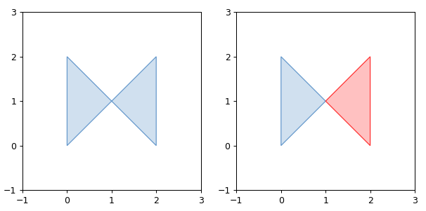
distance = 0
如果距离为 0,buffer() 有时可用于 "清理 "自接触或自交叉的多边形,如经典的 “领结”。用户报告说,很小的距离值有时会产生比 0 更干净的结果。
1
2
3
4
5
6
7
8
9
10
11
12
13
14
15
coords = [(0, 0), (0, 2), (1, 1), (2, 2), (2, 0), (1, 1), (0, 0)] Polygon (coords).is_valid .buffer (0 ).is_valid 0 0 , 0 2 , 1 1 , 0 0 )), ((1 1 , 2 2 , 2 0 , 1 1 )))>len (clean.geoms) 2 list (clean.geoms[0 ].exterior.coords) [(0.0, 0.0), (0.0, 2.0), (1.0, 1.0), (0.0, 0.0)] list (clean.geoms[1 ].exterior.coords) [(1.0, 1.0), (2.0, 2.0), (2.0, 0.0), (1.0, 1.0)]
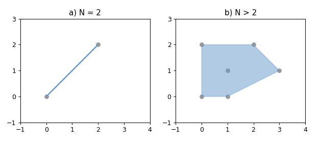
convex_hull 返回包含对象中所有点的最小凸多边形的表示,除非对象中的点数少于三个。对于两个点,凸包折叠成一个 LineString;对于 1,一个点。
示例代码
1
2
3
4
5
6
7
8
9
10
11
12
13
14
15
16
17
18
19
20
21
22
23
24
25
26
27
28
29
30
31
32
33
34
35
import matplotlib.pyplot as pltfrom shapely.geometry import MultiPointfrom shapely.plotting import plot_polygon, plot_line, plot_pointsfrom figures import GRAY, BLUE, SIZE, set_limits1 , figsize=SIZE, dpi=90 )121 )0 , 0 ), (2 , 2 )])False , color=BLUE, zorder=3 )'a) N = 2' )1 , 4 , -1 , 3 )122 )0 , 0 ), (1 , 1 ), (0 , 2 ), (2 , 2 ), (3 , 1 ), (1 , 0 )])False , color=BLUE, zorder=3 , alpha=0.5 )'b) N > 2' )1 , 4 , -1 , 3 )
envelope 返回包含对象的点或最小矩形多边形(边平行于坐标轴)的表示形式。
1 2 3 4 Point(0 , 0 ).envelope0 0 )>0 , 0 ), (1 , 1 )]).envelope0 0 , 1 0 , 1 1 , 0 1 , 0 0 ))>
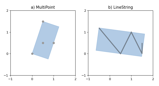
minimum_rotated_rectangle 1 object .minimum_ rotated_ rectangle
返回包含该对象的一般最小外接矩形。与 envelope 不同,该矩形不限于平行于坐标轴。如果对象的凸包是退化维度的图形(线或点),则返回该对象。
示例代码
1
2
3
4
5
6
7
8
9
10
11
12
13
14
15
16
17
18
19
20
21
22
23
24
25
26
27
28
29
30
31
32
33
import matplotlib.pyplot as pltfrom shapely.geometry import MultiPoint, LineStringfrom shapely.plotting import plot_polygon, plot_line, plot_pointsfrom figures import DARKGRAY, GRAY, BLUE, SIZE, set_limits1 , figsize=SIZE, dpi=90 )121 )0 , 0 ), (0.5 , 1.5 ), (1 , 0.5 ), (0.5 , 0.5 )])False , color=BLUE, alpha=0.5 , zorder=-1 )'a) MultiPoint' )1 , 2 , -1 , 2 )122 )0.5 , 1.2 ), (0.5 , 0 ), (1 , 1 ), (1.5 , 0 ), (1.5 , 0.5 )])False , color=DARKGRAY, linewidth=3 , alpha=0.5 )False , color=BLUE, alpha=0.5 , zorder=-1 )1 , 2 , -1 , 2 )'b) LineString' )
多点要素(左)和线串要素(右)的最小旋转矩形。
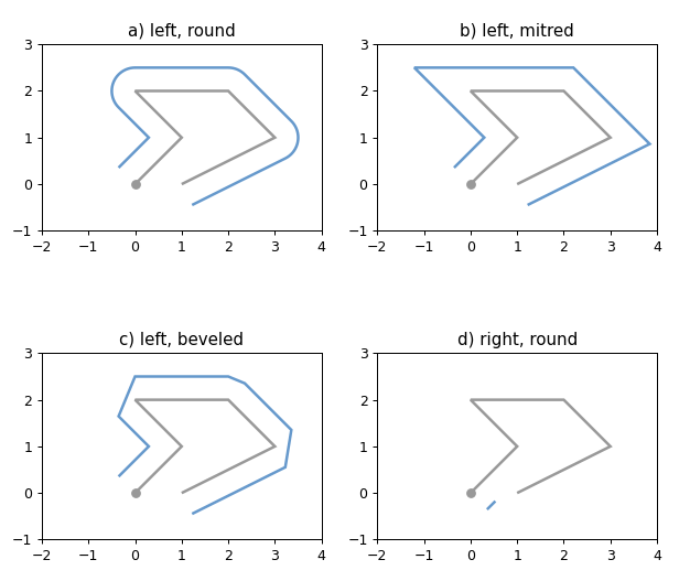
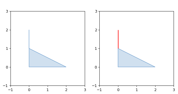
parallel_offset 1 object.parallel_offset(distance, side, resolution =16, join_style =1, mitre_limit =5.0)
返回距其右侧或左侧对象一定距离的 LineString 或 MultiLineString 几何图形。
offset_curve() 方法的较旧替代方法,但使用分辨率而不是quad_segs,并使用 side 关键字(“左”或“右”)而不是距离符号。目前保留此方法是为了向后兼容,但建议使用 offset_curve() 代替。
offset_curve 1 object.offset_curve(distance, quad_segs =16, join_style =1, mitre_limit =5.0)
返回距其右侧或左侧对象一定距离的 LineString 或 MultiLineString 几何图形。
distance 参数必须是浮点值。
边由距离参数的符号确定(负值表示右侧偏移,正值表示左侧偏移)。左和右是通过遵循 LineString 给定几何点的方向来确定的。
对象每个顶点周围偏移的分辨率按照 buffer() 方法(使用quad_segs)进行参数化。
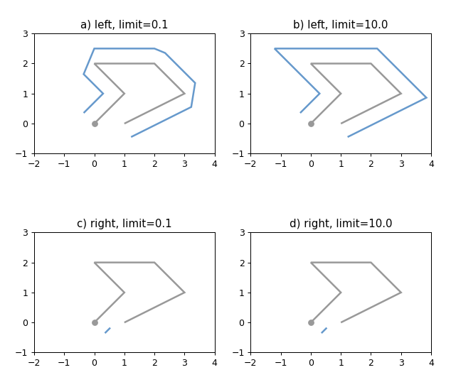
严重斜接的角可以通过 mitre_limit 参数(以英式英语拼写,en-gb)控制。平行线的拐角将比斜接连接样式的大多数地方距原始线更远。该更远的距离与指定距离的比率就是斜接比。比例超过限制的角将会被倒角。
示例代码
1
2
3
4
5
6
7
8
9
10
11
12
13
14
15
16
17
18
19
20
21
22
23
24
25
26
27
28
29
30
31
32
33
34
35
36
37
38
39
40
41
42
43
44
45
46
47
48
49
50
51
52
53
54
55
56
57
58
import matplotlib.pyplot as pltfrom shapely import LineString, get_pointfrom shapely.plotting import plot_line, plot_pointsfrom figures import SIZE, BLUE, GRAY, set_limits0 , 0 ), (1 , 1 ), (0 , 2 ), (2 , 2 ), (3 , 1 ), (1 , 0 )])int (line_bounds[0 ] - 1.0 ), int (line_bounds[2 ] + 1.0 )]int (line_bounds[1 ] - 1.0 ), int (line_bounds[3 ] + 1.0 )]1 , figsize=(SIZE[0 ], 1.5 * SIZE[1 ]), dpi=90 )221 )False , color=GRAY)0 ), ax=ax, color=GRAY)0.5 , 'left' , join_style=1 )False , color=BLUE)'a) left, round' )2 , 4 , -1 , 3 )222 )False , color=GRAY)0 ), ax=ax, color=GRAY)0.5 , 'left' , join_style=2 )False , color=BLUE)'b) left, mitred' )2 , 4 , -1 , 3 )223 )False , color=GRAY)0 ), ax=ax, color=GRAY)0.5 , 'left' , join_style=3 )False , color=BLUE)'c) left, beveled' )2 , 4 , -1 , 3 )224 )False , color=GRAY)0 ), ax=ax, color=GRAY)0.5 , 'right' , join_style=1 )False , color=BLUE)'d) right, round' )2 , 4 , -1 , 3 )
mitre_limit 参数的效果如下所示。
1
2
3
4
5
6
7
8
9
10
11
12
13
14
15
16
17
18
19
20
21
22
23
24
25
26
27
28
29
30
31
32
33
34
35
36
37
38
39
40
41
42
43
44
45
46
47
48
49
50
51
52
53
54
55
56
57
58
import matplotlib.pyplot as pltfrom shapely import LineString, get_pointfrom shapely.plotting import plot_line, plot_pointsfrom figures import SIZE, BLUE, GRAY, set_limits0 , 0 ), (1 , 1 ), (0 , 2 ), (2 , 2 ), (3 , 1 ), (1 , 0 )])int (line_bounds[0 ] - 1.0 ), int (line_bounds[2 ] + 1.0 )]int (line_bounds[1 ] - 1.0 ), int (line_bounds[3 ] + 1.0 )]1 , figsize=(SIZE[0 ], 1.5 * SIZE[1 ]), dpi=90 )221 )False , color=GRAY)0 ), ax=ax, color=GRAY)0.5 , 'left' , join_style=2 , mitre_limit=0.1 )False , color=BLUE)'a) left, limit=0.1' )2 , 4 , -1 , 3 )222 )False , color=GRAY)0 ), ax=ax, color=GRAY)0.5 , 'left' , join_style=2 , mitre_limit=10.0 )False , color=BLUE)'b) left, limit=10.0' )2 , 4 , -1 , 3 )223 )False , color=GRAY)0 ), ax=ax, color=GRAY)0.5 , 'right' , join_style=2 , mitre_limit=0.1 )False , color=BLUE)'c) right, limit=0.1' )2 , 4 , -1 , 3 )224 )False , color=GRAY)0 ), ax=ax, color=GRAY)0.5 , 'right' , join_style=2 , mitre_limit=10.0 )False , color=BLUE)'d) right, limit=10.0' )2 , 4 , -1 , 3 )
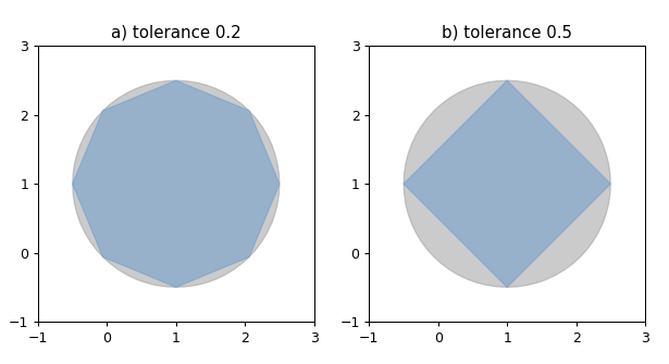
simplify 1 object.simplify(tolerance, preserve_topology =True )
返回几何对象的简化表示。
简化对象中的所有点都将在原始几何体的公差距离内。默认情况下,使用较慢的算法来保留拓扑。如果保留拓扑设置为 False,则使用更快的 Douglas-Peucker 算法 [6]。
示例代码
1
2
3
4
5
6
7
8
9
10
11
12
13
14
15
16
17
18
19
20
21
22
23
24
25
26
27
28
29
30
31
32
33
34
35
import matplotlib.pyplot as pltfrom shapely.geometry import MultiPoint, Pointfrom shapely.plotting import plot_polygonfrom figures import SIZE, BLUE, GRAY, set_limits1 , figsize=SIZE, dpi=90 )1 , 1 ).buffer(1.5 )121 )0.2 )False , color=GRAY, alpha=0.5 )False , color=BLUE, alpha=0.5 )'a) tolerance 0.2' )1 , 3 , -1 , 3 )122 )0.5 )False , color=GRAY, alpha=0.5 )False , color=BLUE, alpha=0.5 )'b) tolerance 0.5' )1 , 3 , -1 , 3 )
使用 0.2(左)和 0.5(右)公差简化近似圆形的多边形。
shapely.affinity 模块中包含仿射变换函数的集合,它通过直接向仿射变换矩阵提供系数或使用特定的命名变换(旋转、缩放等)来返回变换后的几何图形。这些函数可用于所有几何类型(GeometryCollection 除外),并且 3D 仿射变换会保留或支持 3D 类型。
1 shapely.affinity .affine_transform (geom, matrix)
使用仿射变换矩阵返回变换后的几何图形。
系数矩阵以列表或元组的形式提供,分别包含 6 个或 12 个项目,用于 2D 或 3D 变换。
2D
对于 2D 仿射变换,6 个参数矩阵为:
1 [a, b, d, e, xoff, yoff]
表示矩阵:
$$
\begin{split}\begin{bmatrix}
x' \\
y' \\
1
\end{bmatrix} =
\begin{bmatrix}
a & b & x_\mathrm{off} \\
d & e & y_\mathrm{off} \\
0 & 0 & 1
\end{bmatrix}
\begin{bmatrix}
x \\
y \\
1
\end{bmatrix}\end{split}
$$
变换后的坐标方程:
$$
\begin{split}x' &= a x + b y + x_\mathrm{off} \\
y' &= d x + e y + y_\mathrm{off}.\end{split}
$$
3D
对于 3D 仿射变换,12 个参数矩阵为:
1 [a, b, c, d, e, f, g, h, i, xoff, yoff, zoff]
表示矩阵:
$$
\begin{split}\begin{bmatrix}
x' \\
y' \\
z' \\
1
\end{bmatrix} =
\begin{bmatrix}
a & b & c & x_\mathrm{off} \\
d & e & f & y_\mathrm{off} \\
g & h & i & z_\mathrm{off} \\
0 & 0 & 0 & 1
\end{bmatrix}
\begin{bmatrix}
x \\
y \\
z \\
1
\end{bmatrix}\end{split}
$$
变换后的坐标方程:
$$
\begin{split}x' &= a x + b y + c z + x_\mathrm{off} \\
y' &= d x + e y + f z + y_\mathrm{off} \\
z' &= g x + h y + i z + z_\mathrm{off}.\end{split}
$$
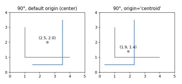
rotate 1 shapely.affinity.rotate(geom, angle, origin ='center' , use_radians =False )
返回 2D 平面上的旋转几何体。
通过设置 use_radians=True 可以以度(默认)或弧度指定旋转角度。正角度是逆时针旋转,负角度是顺时针旋转。
原点可以是边界框中心的关键字 center(默认)、几何体质心的 centroid、Point 对象或坐标元组 (x0, y0)。
二维角度 $\theta$ 旋转的仿射变换矩阵是:
$$
\begin{split}\begin{bmatrix}
\cos{\theta} & -\sin{\theta} & x_\mathrm{off} \\
\sin{\theta} & \cos{\theta} & y_\mathrm{off} \\
0 & 0 & 1
\end{bmatrix}\end{split}
$$
其中偏移量是从点 $(x_0,y_0)$ 计算的:
$$
\begin{split}x_\mathrm{off} &= x_0 - x_0 \cos{\theta} + y_0 \sin{\theta} \\
y_\mathrm{off} &= y_0 - x_0 \sin{\theta} - y_0 \cos{\theta}\end{split}
$$
示例代码 1 2 3 4 5 6 7 8 9 10 11 12 13 14 15 16 17 18 19 20 21 22 23 24 25 26 27 28 29 30 31 32 33 34 import matplotlib.pyplot as pltfrom shapely.geometry import LineStringfrom shapely import affinityfrom shapely.plotting import plot_linefrom figures import SIZE, BLUE, GRAY, set_limits, add_origin1 , figsize=SIZE, dpi=90 )1 , 3 ), (1 , 1 ), (4 , 1 )])121 )False , color=GRAY)90 , 'center' ), ax=ax, add_points=False , color=BLUE)'center' )"90\N{DEGREE SIGN}, default origin (center)" )0 , 5 , 0 , 4 )122 )False , color=GRAY)90 , 'centroid' ), ax=ax, add_points=False , color=BLUE)'centroid' )"90\N{DEGREE SIGN}, origin='centroid'" )0 , 5 , 0 , 4 )
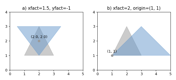
scale 1 shapely.affinity.scale(geom, xfact =1.0, yfact =1.0, zfact =1.0, origin ='center' )
返回缩放后的几何图形,按每个维度上的因子进行缩放。
原点可以是 2D 边界框中心的关键字 center(默认)、几何体 2D 质心的 centroid、Point 对象或坐标元组 (x0, y0, z0)。
负比例因子将镜像或反映坐标。
用于缩放的一般 3D 仿射变换矩阵为:
$$
\begin{split}\begin{bmatrix}
x_\mathrm{fact} & 0 & 0 & x_\mathrm{off} \\
0 & y_\mathrm{fact} & 0 & y_\mathrm{off} \\
0 & 0 & z_\mathrm{fact} & z_\mathrm{off} \\
0 & 0 & 0 & 1
\end{bmatrix}\end{split}
$$
$$
\begin{split}x_\mathrm{off} &= x_0 - x_0 x_\mathrm{fact} \\
y_\mathrm{off} &= y_0 - y_0 y_\mathrm{fact} \\
z_\mathrm{off} &= z_0 - z_0 z_\mathrm{fact}\end{split}
$$
示例代码
1 2 3 4 5 6 7 8 9 10 11 12 13 14 15 16 17 18 19 20 21 22 23 24 25 26 27 28 29 30 31 32 33 34 35 36 37 38 import matplotlib.pyplot as pltfrom shapely.geometry import Polygonfrom shapely import affinityfrom shapely.plotting import plot_polygonfrom figures import SIZE, BLUE, GRAY, set_limits, add_origin1 , figsize=SIZE, dpi=90 )1 , 1 ), (2 , 3 ), (3 , 1 )])121 )False , color=GRAY, alpha=0.5 )1.5 , yfact=-1 )False , color=BLUE, alpha=0.5 )'center' )"a) xfact=1.5, yfact=-1" )0 , 5 , 0 , 4 )122 )False , color=GRAY, alpha=0.5 )2 , origin=(1 , 1 ))False , color=BLUE, alpha=0.5 )1 , 1 ))"b) xfact=2, origin=(1, 1)" )0 , 5 , 0 , 4 )
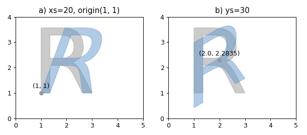
skew 1 shapely.affinity.skew(geom, xs =0.0, ys =0.0, origin ='center' , use_radians =False )
返回一个倾斜的几何体,沿 x 和 y 维度被角度剪切。
通过设置 use_radians=True 可以以度数(默认)或弧度指定剪切角。
原点可以是边界框中心的关键字 center(默认)、几何体质心的 centroid、Point 对象或坐标元组 (x0, y0)。
倾斜的一般二维仿射变换矩阵为:
$$
\begin{split}\begin{bmatrix}
1 & \tan{x_s} & x_\mathrm{off} \\
\tan{y_s} & 1 & y_\mathrm{off} \\
0 & 0 & 1
\end{bmatrix}\end{split}
$$
$$
\begin{split}x_\mathrm{off} &= -y_0 \tan{x_s} \\
y_\mathrm{off} &= -x_0 \tan{y_s}\end{split}
$$
示例代码
1 2 3 4 5 6 7 8 9 10 11 12 13 14 15 16 17 18 19 20 21 22 23 24 25 26 27 28 29 30 31 32 33 34 35 36 37 38 39 40 41 42 43 44 45 46 47 48 49 50 51 import matplotlib.pyplot as pltfrom shapely.wkt import loads as load_wktfrom shapely import affinityfrom shapely.plotting import plot_polygonfrom figures import SIZE, BLUE, GRAY, set_limits, add_origin1 , figsize=SIZE, dpi=90 )'''\ POLYGON((2.218 2.204, 2.273 2.18, 2.328 2.144, 2.435 2.042, 2.541 1.895, 2.647 1.702, 3 1, 2.626 1, 2.298 1.659, 2.235 1.777, 2.173 1.873, 2.112 1.948, 2.051 2.001, 1.986 2.038, 1.91 2.064, 1.823 2.08, 1.726 2.085, 1.347 2.085, 1.347 1, 1 1, 1 3.567, 1.784 3.567, 1.99 3.556, 2.168 3.521, 2.319 3.464, 2.441 3.383, 2.492 3.334, 2.536 3.279, 2.604 3.152, 2.644 3.002, 2.658 2.828, 2.651 2.712, 2.63 2.606, 2.594 2.51, 2.545 2.425, 2.482 2.352, 2.407 2.29, 2.319 2.241, 2.218 2.204), (1.347 3.282, 1.347 2.371, 1.784 2.371, 1.902 2.378, 2.004 2.4, 2.091 2.436, 2.163 2.487, 2.219 2.552, 2.259 2.63, 2.283 2.722, 2.291 2.828, 2.283 2.933, 2.259 3.025, 2.219 3.103, 2.163 3.167, 2.091 3.217, 2.004 3.253, 1.902 3.275, 1.784 3.282, 1.347 3.282))''' )121 )False , color=GRAY, alpha=0.5 )20 , origin=(1 , 1 ))False , color=BLUE, alpha=0.5 )1 , 1 ))"a) xs=20, origin(1, 1)" )0 , 5 , 0 , 4 )122 )False , color=GRAY, alpha=0.5 )30 )False , color=BLUE, alpha=0.5 )'center' )"b) ys=30" )0 , 5 , 0 , 4 )
translate 1 shapely .affinity.translate(geom, xoff=0 .0 , yoff=0 .0 , zoff=0 .0 )
返回沿每个维度按偏移量移动的平移几何图形。
一般用于平移的 3D 仿射变换矩阵为:
$$
\begin{split}\begin{bmatrix}
1 & 0 & 0 & x_\mathrm{off} \\
0 & 1 & 0 & y_\mathrm{off} \\
0 & 0 & 1 & z_\mathrm{off} \\
0 & 0 & 0 & 1
\end{bmatrix}\end{split}
$$
Shapely 支持地图投影和几何对象的其他任意变换。
1 shapely.ops .transform (func, geom)
将 func 应用于 geom 的所有坐标,并从转换后的坐标返回相同类型的新几何图形。
func 将 x、y 和(可选的 z)映射到输出 xp、yp、zp。输入参数可以是可迭代类型,例如列表或数组或单个值。输出应具有相同类型:标量输入,标量输出;列出,列出。
首先,transform 尝试通过使用 n 个可迭代的坐标调用 func 来确定传入的函数类型,其中 n 是输入几何图形的维数。如果 func 在使用可迭代对象作为参数调用时引发 TypeError,那么它将改为在几何图形中的每个单独坐标上调用 func。
例如,这是一个适用于两种类型的输入(标量或数组)的恒等函数。
1
2
3
4
def id_func (x, y, z=None ):return tuple (filter (None , [x, y, z]))
如果使用 pyproj>=2.1.0,投影几何图形的首选方法是:
1
2
3
4
5
6
7
8
9
10
11
12
import pyprojfrom shapely import Pointfrom shapely.ops import transform72.2495 , 43.886 )'EPSG:4326' )'EPSG:32618' )True ).transform
官方文档
其他功能 (Other Operations)
合并线性特征(Merging Linear Features)
可以使用 shapely.ops 模块中的函数将接触线序列合并到 MultiLineStrings 或 Polygons 中。
polygonize 1 shapely.ops .polygonize (lines)
返回根据输入线构造的多边形的迭代器。
与 MultiLineString 构造函数一样,输入元素可以是任何类似行的对象。
1
2
3
4
5
6
7
8
9
10
from shapely.ops import polygonize0 , 0 ), (1 , 1 )),0 , 0 ), (0 , 1 )),0 , 1 ), (1 , 1 )),1 , 1 ), (1 , 0 )),1 , 0 ), (0 , 0 ))list (polygonize(lines))0 0 , 1 1 , 1 0 , 0 0 ))>, <POLYGON ((1 1 , 0 0 , 0 1 , 1 1 ))>]
polygonize_full 1 shapely.ops .polygonize_full (lines)
从线源创建多边形,返回多边形和剩余的几何图形。
源可以是 MultiLineString、LineString 对象序列或可适应 LineString 的对象序列。
返回对象元组:(多边形、切边、悬垂物、无效环线)。每一个都是一个几何集合。
悬空是指一端或两端不与另一边端点重合的边。切边在两端相连,但不形成多边形的一部分。无效的环线形成无效的环(领结等)。
1
2
3
4
5
6
7
8
9
10
11
12
13
14
15
16
17
from shapely.ops import polygonize_full0 , 0 ), (1 , 1 )),0 , 0 ), (0 , 1 )),0 , 1 ), (1 , 1 )),1 , 1 ), (1 , 0 )),1 , 0 ), (0 , 0 )),5 , 5 ), (6 , 6 )),1 , 1 ), (100 , 100 )),len (result.geoms)2 list (result.geoms)0 0 , 1 1 , 1 0 , 0 0 ))>, <POLYGON ((1 1 , 0 0 , 0 1 , 1 1 ))>]list (dangles.geoms)1 1 , 100 100 )>, <LINESTRING (5 5 , 6 6 )>]
linemerge 1 shapely.ops .linemerge (lines)
返回表示行的所有连续元素的合并的 LineString 或 MultiLineString。
与 shapely.ops.polygonize() 一样,输入元素可以是任何线状对象。
1
2
3
4
5
6
7
8
9
from shapely.ops import linemerge1 1 , 1 0 , 0 0 ), (0 0 , 1 1 ), (0 0 , 0 1 , 1 1 ), (1 1 , 100 10. ..>list (linemerge(lines).geoms)1 1 , 1 0 , 0 0 )>,0 0 , 1 1 )>,0 0 , 0 1 , 1 1 )>,1 1 , 100 100 )>,5 5 , 6 6 )>]
高效矩形裁剪 (Efficient Rectangle Clipping)
shapely.ops 中的 clip_by_rect() 函数返回矩形内几何图形的部分。
1 shapely.ops .clip_by_rect (geom, xmin, ymin, xmax, ymax)
几何体以快速但可能出问题的方式被剪裁。不保证输出有效。拓扑错误不会引发任何异常。
1
2
3
4
5
6
7
8
from shapely.ops import clip_by_rect0 , 0 ), (0 , 30 ), (30 , 30 ), (30 , 0 ), (0 , 0 )],10 , 10 ), (20 , 10 ), (20 , 20 ), (10 , 20 ), (10 , 10 )]],5 , 5 , 15 , 15 )5 5 , 5 15 , 10 15 , 10 10 , 15 10 , 15 5 , 5 5 ))>
高效并集运算 (Efficient Unions)
shapely.ops 中的 unary_union() 函数比使用 union() 累加更高效。
unary_union
1 shapely.ops .unary_union (geoms)
返回给定几何对象的并集的表示。
重叠多边形的区域将被合并。 LineStrings 将完全溶解并节点化。重复的点将被合并。
示例代码
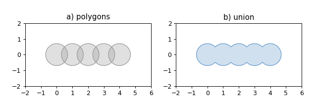
1
2
3
4
5
6
7
8
9
10
11
12
13
14
15
16
17
18
19
20
21
22
23
24
25
26
27
28
29
30
31
32
import matplotlib.pyplot as pltfrom shapely.geometry import Pointfrom shapely.ops import unary_unionfrom shapely.plotting import plot_polygonfrom figures import SIZE, BLUE, GRAY, set_limits0 ).buffer(0.7 ) for i in range (5 )]1 , figsize=SIZE, dpi=90 )121 )for ob in polygons:False , color=GRAY)'a) polygons' )2 , 6 , -2 , 2 )122 )False , color=BLUE)'b) union' )2 , 6 , -2 , 2 )
因为联合合并了重叠多边形的区域,所以它可以用于尝试修复无效的多多边形。与零距离 buffer() 技巧一样,使用此技巧时您的里程可能会有所不同。
1
2
3
4
5
6
7
8
9
m = MultiPolygon(polygons)7.684543801837549 False 6.610301355116799 True
cascaded_union 1 shapely.ops .cascaded_union (geoms)
返回给定几何对象的并集的表示。
德劳内三角 (Delaunay triangulation)
1 shapely.ops.triangulate(geom, tolerance =0.0, edges =False )
shapely.ops 中的 triangulate() 函数根据点集合计算 Delaunay 三角剖分。
返回输入几何体顶点的 Delaunay 三角剖分。
示例代码
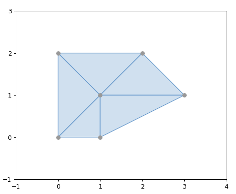
1
2
3
4
5
6
7
8
9
10
11
12
13
14
15
16
17
18
19
20
21
22
import matplotlib.pyplot as pltfrom shapely.geometry import MultiPointfrom shapely.ops import triangulatefrom shapely.plotting import plot_polygon, plot_pointsfrom figures import SIZE, BLUE, GRAY, set_limits0 , 0 ), (1 , 1 ), (0 , 2 ), (2 , 2 ), (3 , 1 ), (1 , 0 )])1 , figsize=SIZE, dpi=90 )111 )for triangle in triangles:False , color=BLUE)1 , 4 , -1 , 3 )
沃罗诺图 (Voronoi Diagram)
1 shapely.ops.voronoi_diagram(geom, envelope =None, tolerance =0.0, edges =False )
shapely.ops 中的 voronoi_diagram() 函数根据集合点或任何几何体的顶点构造 Voronoi 图。
从输入几何体的顶点构造 Voronoi 图。
示例代码
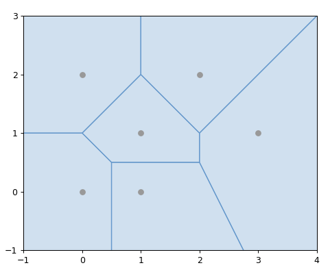
1
2
3
4
5
6
7
8
9
10
11
12
13
14
15
16
17
18
19
20
21
22
import matplotlib.pyplot as pltfrom shapely.geometry import MultiPointfrom shapely.ops import voronoi_diagramfrom shapely.plotting import plot_polygon, plot_pointsfrom figures import SIZE, BLUE, GRAY, set_limits0 , 0 ), (1 , 1 ), (0 , 2 ), (2 , 2 ), (3 , 1 ), (1 , 0 )])1 , figsize=SIZE, dpi=90 )111 )for region in regions.geoms:False , color=BLUE)1 , 4 , -1 , 3 )
最近点(Nearest points)
1 shapely.ops .nearest_points (geom1, geom2)
返回输入几何中最近点的元组。点的返回顺序与输入几何图形的顺序相同。
1
2
3
4
5
from shapely.ops import nearest_pointstriangle = Polygon([(0 , 0 ), (1 , 0 ), (0 .5 , 1 ), (0 , 0 )])square = Polygon([(0 , 2 ), (1 , 2 ), (1 , 3 ), (0 , 3 ), (0 , 2 )])list (nearest_points(triangle, square))[<POINT (0.5 1)>, <POINT (0.5 2)>]
请注意,最近的点可能不是几何图形中的现有顶点。
捕捉 (Snapping)
1 shapely.ops .snap (geom1, geom2, tolerance)
将 geom1 中的顶点捕捉到 geom2 中的顶点。返回捕捉的几何体的副本。输入几何形状未修改。
容差参数指定要捕捉的顶点之间的最小距离。
1
2
3
4
5
6
from shapely.ops import snap1 ,1 ), (2 , 1 ), (2 , 2 ), (1 , 2 ), (1 , 1 )])0 ,0 ), (0.8 , 0.8 ), (1.8 , 0.95 ), (2.6 , 0.5 )])0.5 )0 0 , 1 1 , 2 1 , 2.6 0.5 )>
共享路径 (Shared paths)
1 shapely.ops .shared_paths (geom1, geom2)
查找 geom1 和 geom2 之间的共享路径,其中两个几何图形都是 LineString。
1
2
3
4
5
6
7
8
from shapely.ops import shared_paths0 , 0 ), (10 , 0 ), (10 , 5 ), (20 , 5 )])5 , 0 ), (30 , 0 ), (30 , 5 ), (0 , 5 )])5 0 , 10 0 ))>10 5 , 20 5 ))>
分割 (Splitting)
1 shapely.ops .split (geom, splitter)
将一个几何图形分割为另一个几何图形并返回几何图形的集合。该函数在理论上与分割几何部分的并集相反。如果分割器不分割几何图形,则返回具有等于输入几何图形的单个几何图形的集合。
1
2
3
4
5
6
from shapely.ops import split1 , 1 ))0 ,0 ), (2 ,2 )])0 0 , 1 1 ), LINESTRING (1 1 , 2 2 ))>
子串 (Substring)
1 shapely.ops .substring (geom, start_dist, end_dist[, normalized=False] )
返回 start_dist 和 end_dist 之间的 LineString 或 Point(如果它们位于同一位置)
1
2
3
4
5
6
7
8
9
10
11
12
13
14
15
from shapely.ops import substring0 ) for i in range (6 ))0 0 , 1 0 , 2 0 , 3 0 , 4 0 , 5 0 )>1 , end_dist=3 )1 0 , 2 0 , 3 0 )>3 , end_dist=1 )3 0 , 2 0 , 1 0 )>1 , end_dist=-3 )1 0 , 2 0 )>0.2 , end_dist=-0.6 , normalized=True )1 0 , 2 0 )>2.5 , end_dist=-2.5 )2.5 0 )>
准备的几何操作(Prepared Geometry Operations)
创建并返回准备好的几何对象。prepared.prep() 函数。
1
2
3
4
5
6
7
from shapely.prepared import prep0.0 , 0.0 ).buffer(1.0 )object at 0x...>filter (prepared_polygon.contains, points)
Prepared geometries 实例具有以下方法:contains、contains_properly、covers 和 intersects。所有这些都与未准备的几何对象中的对应对象具有完全相同的参数和用法。
诊断 (Diagnostics)
explain_validity
1 validation.explain_validity (ob)
返回一个字符串,解释对象的有效性或无效性。
1
2
3
4
5
coords = [(0 , 0 ), (0 , 2 ), (1 , 1 ), (2 , 2 ), (2 , 0 ), (1 , 1 ), (0 , 0 )]from shapely.validation import explain_validity'Ring Self-intersection[1 1]'
make_valid 1 validation.make_valid (ob)
如果几何图形无效,则返回有效的表示形式。如果有效,将返回输入的几何图形。
在许多情况下,为了创建有效的几何图形,必须将输入几何图形分割成多个部分或多个几何图形。如果必须将几何图形分割成相同几何类型的多个部分,则将返回多部分几何图形(例如 MultiPolygon)。如果必须将几何图形拆分为不同类型的多个部分,则将返回 GeometryCollection。
示例代码
1
2
3
4
5
6
7
8
9
10
11
12
13
14
15
16
17
18
19
20
21
22
23
24
25
26
27
import matplotlib.pyplot as pltfrom shapely.geometry import Polygonfrom shapely.validation import make_validfrom shapely.plotting import plot_polygonfrom figures import SIZE, BLUE, RED, set_limits0 , 0 ), (0 , 2 ), (1 , 1 ), (2 , 2 ), (2 , 0 ), (1 , 1 ), (0 , 0 )])1 , figsize=SIZE, dpi=90 )121 )False , color=BLUE)1 , 3 , -1 , 3 )122 )0 ], ax=valid_ax, add_points=False , color=BLUE)1 ], ax=valid_ax, add_points=False , color=RED)1 , 3 , -1 , 3 )
1
2
3
4
5
6
7
8
9
10
11
12
13
14
15
16
17
18
19
20
21
22
23
24
25
26
27
28
import matplotlib.pyplot as pltfrom shapely.geometry import Polygonfrom shapely.validation import make_validfrom shapely.plotting import plot_polygon, plot_linefrom figures import SIZE, BLUE, RED, set_limits0 , 2 ), (0 , 1 ), (2 , 0 ), (0 , 0 ), (0 , 2 )])1 , figsize=SIZE, dpi=90 )121 )False , color=BLUE)1 , 3 , -1 , 3 )122 )0 ], ax=valid_ax, add_points=False , color=BLUE)1 ], ax=valid_ax, add_points=False , color=RED)1 , 3 , -1 , 3 )
Polylabel
1 shapely.ops .polylabel (polygon, tolerance)
查找给定多边形的不可到达极点的大致位置。基于弗拉基米尔·阿加丰金 (Vladimir Agafonkin) 的 Polylabel 。
1
2
3
4
5
6
from shapely.ops import polylabel0 , 0 ), (50 , 200 ), (100 , 100 ), (20 , 50 ),100 , -20 ), (-150 , -200 )]).buffer(100 )10 )59.356 121.839 )>
交互 (Interoperation)
Shapely 提供了 4 种与其他软件互操作的途径。
任何几何对象的众所周知的文本(WKT)或众所周知的二进制(WKB)表示都可以通过其 wkt 或 wkb 属性获得。这些表示允许与许多 GIS 程序互换。例如,PostGIS 以十六进制编码的 WKB 进行交互。
1 2 3 4 5 6 Point(0 , 0 ).wkt'POINT (0 0)' 0 , 0 ).wkbb'\x01\x01\x00\x00\x00\x00\x00\x00\x00\x00\x00\x00\x00\x00\x00\x00\x00\x00\x00\x00\x00' 0 , 0 ).wkb_hex'010100000000000000000000000000000000000000'
shapely.wkt和shapely.wkb模块提供了dumps()和loads()函数,它们的工作方式几乎与pickle和simplejson模块的对应函数完全相同。要将几何对象序列化为二进制或文本字符串,请使用 dumps()。要反序列化字符串并获取适当类型的新几何对象,请使用loads()。
wkt 属性和 shapely.wkt.dumps() 函数的默认设置不同。默认情况下,该属性的值会修剪掉多余的小数,而 dumps() 则不是这种情况,尽管可以通过设置 trim=True 来复制它。
返回 ob 的 WKB 表示形式。
从 WKB 表示形式 wkb 返回一个几何对象。
1
2
3
4
5
6
7
8
from shapely import wkb0 , 0 )b'\x01\x01\x00\x00\x00\x00\x00\x00\x00\x00\x00\x00\x00\x00\x00\x00\x00\x00\x00\x00\x00' b'\x01\x01\x00\x00\x00\x00\x00\x00\x00\x00\x00\x00\x00\x00\x00\x00\x00\x00\x00\x00\x00' 'POINT (0 0)'
Numpy and Python Arrays
所有具有坐标序列的几何对象(Point、LinearRing、LineString)都提供 Numpy 数组接口,从而可以转换或适应 Numpy 数组。
1
2
3
4
5
6
import numpy as np0 , 0 ).coords)0. , 0. ]])0 , 0 ), (1 , 1 )]).coords)0. , 0. ],1. , 1. ]])
相同类型的几何对象的坐标可以通过 xy 属性作为 x 和 y 值的标准 Python 数组。
1 2 3 4 Point(0 , 0 ).xy'd' , [0.0 ]), array('d' , [0.0 ]))0 , 0 ), (1 , 1 )]).xy'd' , [0.0 , 1.0 ]), array('d' , [0.0 , 1.0 ]))
Python Geo Interface
任何提供类似 GeoJSON 的 Python 地理接口的对象都可以使用 shapely.geometry.shape() 函数转换为 Shapely 几何图形。
1 shapely.geometry .shape (context)
返回一个新的独立几何体,其坐标是从上下文复制的。
1
2
3
4
5
6
7
8
9
10
11
12
13
14
15
16
17
from shapely.geometry import shape"type" : "Point" , "coordinates" : (0.0 , 0.0 )}'Point' list (geom.coords)0.0 , 0.0 )]class GeoThing :def __init__ (self, d ):"type" : "Point" , "coordinates" : (0.0 , 0.0 )})'Point' list (geom.coords)0.0 , 0.0 )]
可以使用 shapely.geometry.mapping() 获得几何对象的类似 GeoJSON 的映射。
1 shapely.geometry .mapping (ob)
从 Geometry 或任何实现 geo_interface 的对象返回类似 GeoJSON 的映射。
1
2
3
4
5
6
7
from shapely.geometry import mapping"type" : "Point" , "coordinates" : (0.0 , 0.0 )})'type' ]'Point' 'coordinates' ]0.0 , 0.0 )
参考资料
文章链接:https://www.zywvvd.com/notes/coding/python/shapely/shapely-user-manual-204/