本文最后更新于:2025年4月30日 下午
Open3D 是一个开源库,用于处理3D数据的快速开发。它由一家名为Syntechsis的公司开发,并得到了社区的广泛支持。Open3D 提供了一系列的3D数据处理功能,本文记录基础用法。
简介
Open3D 是一个开源库,支持快速开发处理3D 数据的软件。Open3D 前端用 C + + 和 Python 公开了一组精心挑选的数据结构和算法。后端是高度优化的,并为并行化而设置。
官方网站:https://www.open3d.org/
点云格式
常见点云存储方式有 pcd、ply、txt、bin文件,下面分别对其进行介绍。
pcd
pcd点云格式是pcl库种常常使用的点云文件格式。一个pcd文件中通常由两部分组成:分别是文件说明和点云数据。 文件说明由11行组成,如下所示。
1
2
3
4
5
6
7
8
9
10
11
.PCD v0.7 - Point Cloud Data file format 4 4 4 1 1 1 35947 1 0 0 0 1 0 0 0 35947
从第12行开始为点云数据,每个点与上面的FIELDS相对应。一般来说,就的点云的x,y,z坐标。pcd格式的点云可视化由于其组成就是xyz坐标,所以可以使用mayavi.mlab来直接显示:mlab.points3d(x, y, z,y, mode=“point”)
1 2 3 4 5 6 7 ps:pcd文件的读取方式如下所示lines = []with open (file_path, 'r' ) as f:lines = f.readlines()return lines
ply
一个ply文件中通常由两部分组成:分别是文件说明和点云数据。这与pcd文件很像。 文件说明如下组成,如下所示。前3行与最后1行是描述性语句,中间部分主要说明每一行存储的是什么样的数据、数据的数量、属性等。定义元素的组成需要用到element和property两部分,第一部分element定义元素名称和数量,第二部分property逐一列举元素组成和类型。
下面的示例中定义了点的存储名称为vertex,共35947个。后面存储每一个点含5个属性,即每一行由5个数组成;然后定义了面的存储名称是face,共69451个。后面存储每一个面含1个属性,这个属性是一个列表,存储的是每一个点的索引。
文件从end_header结束后为点云数据,每一行存储的数据与element对应,描述结束。随后开始逐一按行列举上述两种元素,第一种元素是35947个点,每行有5个属性,共35947行。第二中元素是69451个面,每行1个属性,共69451行。
1 2 3 4 5 6 7 8 9 10 11 12 13 14 15 16 plyformat ascii 1.0 35947 property float x property float y property float z property float confidence property float intensity 69451 property list uchar int vertex_indices 0.0378297 0.12794 0.00447467 0.850855 0.5 0.0447794 0.128887 0.00190497 0.900159 0.5 0.0680095 0.151244 0.0371953 0.398443 0.5 0.00228741 0.13015 0.0232201 0.85268 0.5
对于ply文件合适内容,点云的每个点由5个属性构成,前三个属性也是xyz的坐标位置。将xyz坐标提取出来,即可利用mlab进行3d绘图。而描述面属性的数据在可视化操作中是不需要使用到的,所以直接提取描述点的35947行数据即可。如下代码所示:points = pcd_read(file_path)[12:(12+35947)],这里的第12行开始,到之后的35947+12行结束,都是描述点的数据。
ply格式的文件读取方式同pcd格式,不能直接使用numpy.fromfile来读取,只可以通过open函数读取,随后进行一定的数据处理。读取方式:
1
2
3
4
5
6
def pcd_read(file_path):lines = []with open (file_path, 'r' ) as f:lines = f.readlines()return lines
txt
txt文件可以说是最朴素简单的点云描述文件了。 txt点云文件与前两篇介绍的pcd和ply点云格式的区别在于,其通常只含点云信息,不含文件说明部分。txt格式的点云文件中的每一行代表一个点,文件中行数即为点的数量。每行数据全部是点的数据,不包含任何的描述信息。行的取值可以是以下几种形式数据的排列组合。
(1)x、y、z:点云的空间坐标。
(2)i:强度值,强度反应了点的密集成度。
(3)r、g、b:rgb色彩信息。
(4)a:a代表alpha(透明度)。
(5)nx、ny、nz:n代表Normal,点云的法向量。
以Pointnet的modelnet40为例,其点云表示方式如下所示x、y、z、normal_x、normal_y、normal_z。样例如下所示:
1
2
3
4
5
6
# 每一行代表一个点的数据0.208700,0 .221100,0 .565600,0 .837600 ,-0.019280 ,0.545900 0.404700 ,0.080140 ,-0.002638 ,0.002952 ,0.973500 ,-0.228800 0.043890 ,-0.115500 ,-0.412900 ,-0.672800 ,0.679900 ,-0.291600 0.525000 ,0.158200,0 .303300,0 .000000 ,-0.413200,0 .910600 0.191700 ,-0.160900,0 .657400,0 .228400 ,-0.071910 ,0.970900
同样的,由于是txt文件,所以直接使用简单的numpy即可读取txt文件,而上述的pcd,ply需要用open函数的系统操作读取。txt文件的同样只需要读取其xyz坐标信息即可。
读取方式:np.loadtxt()
1
2
txt_file = r"E:\workspace\PointCloud\Pointnet2\data\modelnet40_normal_resampled\airplane\airplane_0001.txt" ',' )
bin
bin文件的存储方式是以二进制形式存储,这带来的好处是读写的速度快,精度不丢失。与txt文件相同,其没有文件的描述信息,只包含点云数据,没有文件的说明部分。但是,txt文件按行存储点的信息,而bin则是将全部数据合并为一个序列,也可以理解为一行。也就是说,读取一个bin文件的输出是一个长串的序列信息,一般需要将其reshape一下,每4个数据为一个点云数据,所以需要reshape成N行4列。样例如下所示:
1
2
3
4
5
6
7
8
9
10
49 .52 22 .668 2 .051 0 . 49 .428 22 .814 2 .05 0 . 48 .096 22 .658 2 .007 0 .05 47 .813 22 .709 1 .999 0 . 48 .079 23 .021 2 .012 0 .48 .211 23 .271 2 .019 0 . 46 .677 22 .71 1 .964 0 . 46 .437 22 .774 1 .958 0 .12 46 .075 22 .776 1 .947 0 .18 45 .994 22 .826 1 .945 0 .18 45 .881 22 .95 1 .944 0 .23 45 .721 23 .05 1 .941 0 . 45 .763 23 .252 1 .945 0 .12 45 .617 23 .358 1 .942 0 .12 45 .667 23 .565 1 .947 0 .16 45 .65 23 .738 1 .949 0 .28 45 .586 23 .796 1 .948 0 .11 45 .591 23 .981 1 .951 0 . 48 .238 25 .569 2 .055 0 .05 43 .789 23 .385 1 .888 0 .14 43 .779 23 .556 1 .89 0 . 43 .784 23 .737 1 .893 0 . 43 .719 23 .88 1 .894 0 . 43 .987 24 .116 1 .905 0 . 43 .024 23 .763 1 .871 0 .
bin文件reshape之后的4列依次是x,y,z的坐标位置,以及反映强度s。所以,直接提取前3列即可用mlab来实现点云的可视化操作。读取方式:np.fromfile()
1
2
kitti_file = r'E:\Study\Machine Learning\Dataset3d\kitti\training\velodyne\000100.bin' 1 ).reshape([-1 , 4 ])
总结:以上既是点云数据的4中常见的数据格式,pcd和ply格式具有说明文档,txt和bin格式没有说明文档更加直观。
Open3d读写点云
pcd 格式
Open3d 读取到的点云通常存储到PointCloud类中。
对于点云矩阵,通常要转换为PointCloud格式才能被Open3d处理,包括存储和点云处理等。
1
2
3
4
5
import numpy as npimport open3d35947 , 3 )
Open3d读取pcd格式点云文件的函数为o3d.io.read_point_cloud,读取的点云存储为上图所示的PointCloud类
1
2
3
4
import open3d as o3dimport numpy as np
保存点云文件的函数为o3d.io.write_point_cloud
1
2
3
import open3d as o3dTrue )
ply 格式
open3d处理ply数据与处理pcd数据是类似的,只是在open3d处理ply数据是转化为TriangleMesh格式,包括存储和点云处理等。也就是说,对于ply点云文件,Open3d读取到的点云通常存储到TriangleMesh类中,vertices存储了全部的点云坐标。
1
2
3
import open3d as o3d
1
2
3
4
5
import open3dimport numpy as npr"E:\Study\Machine Learning\Dataset3d\points_ply\lucy\lucy.ply"
1
2
3
import open3d as o3dTrue )
点云格式的转换
在mmdetection3d中提供了一些点云格式转换的工具代码。
1
2
3
4
5
6
7
8
9
10
11
12
13
14
import numpy as npimport pandas as pdfrom plyfile import PlyDatadef convert_ply (input_path, output_path ):0 ].data float ) 0 ].dtype.names for i, name in enumerate ('./test.ply' , './test.bin' )
如果你有其他格式的点云文件 (例:off, obj), 你可以使用 trimesh 将它们转化成 ply.
1
2
3
4
5
6
import trimeshdef to_ply (input_path, output_path, original_type ):'ply' ) './test.obj' , './test.ply' , 'obj' )
Open3d 配准点云
点云配准本质上是将点云从一个坐标系变换到另一个坐标系。点云配准通常会需要用到两个点云数据。第一类点云数据称为原始点云,用S(source)来表示。第二类点云数据称为目标点云,用T(Target)来表示。配准就是希望这里的原始数据可以对其目标数据的坐标系,让原始点云S在目标点云T的坐标上进行显示。以实现数据的补充。我们可以通过找到点云中具有相似特征的点云来确定坐标的变换关系。例如,同一个物体的点云同时出现在原始点云和目标点云中,并且在两个点云中有特征相似的部分点云,根据这些相似的点云信息来计算出变换关系。
假设原始点云到目标点云发生的是刚体变换,即原始点云通过旋转和平移即可得到目标点云。这里的旋转和平移过程用旋转变换矩阵R和平移变换矩阵T来表示。我们用P(S)表示原始点云中的点,P(T)表示原始点云在目标点云坐标系中的点。那么这种变换关系可以表示为:
迭代最近点算法 (Iterative Closest Point, ICP)
第一步:初始化R、T矩阵,根据R、T矩阵可以得到P(T),即原始点云在目标点云坐标系下的坐标。
第二步:在目标点云中寻找与P(T)最近的点,并且距离小于规定的阈值,这个阈值可以自己定义。
第三步:对第二步中匹配到的点计算欧式距离误差,并且通过最小二乘法来优化R、T矩阵。
第四步:将第三步优化后的R、T矩阵带回第一步中,重新进行迭代,直到迭代满足要求后,得到最终优化的R、T矩阵。
ICP方法可分为点到点(PointToPoint)和点到平面(PointToPlane)两类。
1)PointToPoint:计算P(t)和目标点云T的距离采用点到点之间的距离形式。
2)PointToPlane:计算P(t)中点到目标点云T的点所在平面的距离,这里通常需要用到目标点云的法向量。
Open3d 配准实现
在Open3d的open3d.pipelines.registration中,提供了几种点云配准的方法。
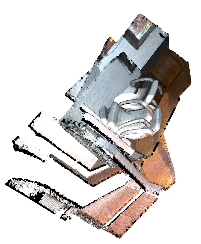
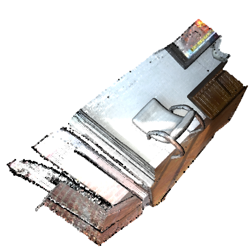
在下面的参考代码中,就是使用了open3d.pipelines.registration这个函数来实现原始点云到目标点云上的配准。参考代码中的happyStandRight_0.ply作为原始点云,对应代码中的point_s1,结果中显示绿色部分点云;happyStandRight_24.ply作为目标点云,对应代码中的point_s2,结果中显示红色部分;原始点云在目标点云上的配准是显示蓝色部分。(以上的颜色是通过控制参数color来实现的)
参考代码:
1
2
3
4
5
6
7
8
9
10
11
12
13
14
15
16
17
18
19
20
21
22
23
24
25
26
27
28
29
30
31
32
33
34
35
36
37
38
39
40
41
42
43
import open3dimport numpy as npimport mayavi.mlab as mlabdef open3d_registration ():r"E:\Study\Machine Learning\Dataset3d\points_ply\happy_stand\happyStandRight_0.ply" r"E:\Study\Machine Learning\Dataset3d\points_ply\happy_stand\happyStandRight_24.ply" print (point_s1.shape, point_s2.shape)0.2 , print (icp)0 ]1 ]2 ]0 , 0 , 0 ), size=(640 , 640 ))"point" , color=(0 , 0 , 1 ), figure=fig) 0 ]1 ]2 ]"point" , color=(0 , 1 , 0 ), figure=fig) 0 ]1 ]2 ]"point" , color=(1 , 0 , 0 ), figure=fig) if __name__ == '__main__' :
ps: 这里的 print(icp) 会计算两个重要指标
1)fitness计算重叠区域(内点对应关系/目标点数),越高越好(但也存在匹配错误但是重合度更高的情况)。
2)inlier_rmse计算所有内在对应关系的均方根误差RMSE,越低越好(可以作为最小二乘法的优化指标)。
Open3D 多点云配准
多个点云的配准方法 Multiway registration
官方文档:https://www.open3d.org/docs/release/tutorial/pipelines/multiway_registration.html
可以下载 示例点云文件 ,解压文件得到 cloud_bin_0.pcd、cloud_bin_1.pcd、cloud_bin_2.pcd
1
2
3
4
5
6
7
8
9
10
11
12
13
14
15
16
17
18
19
20
21
22
23
24
25
26
27
28
29
30
31
32
33
34
35
36
37
38
39
40
41
42
43
44
45
46
47
48
49
50
51
52
53
54
55
56
57
58
59
60
61
62
63
64
65
66
67
68
69
70
71
72
73
74
75
76
77
78
79
80
81
82
83
84
85
86
87
88
89
90
91
92
93
94
95
96
97
98
99
100
101
102
103
104
105
106
107
108
109
110
111
112
113
114
115
116
117
118
119
120
121
122
import open3d as o3dimport numpy as npdef pairwise_registration (source, target, max_correspondence_distance_coarse, max_correspondence_distance_fine, method= 'Point2Point' ):if method == 'Point2Point' :elif method == 'Point2Plane' :else :raise ValueError("Invalid method. Use 'Point2Point' or 'Point2Plane'" )print ("Apply point-to-plane ICP" )4 ),200 ))200 ))return transformation_icp, information_icpdef full_registration (pcds, max_correspondence_distance_coarse, max_correspondence_distance_fine, method='Point2Point' ):4 )len (pcds)for source_id in range (n_pcds):for target_id in range (source_id + 1 , n_pcds):print ("Build o3d.pipelines.registration.PoseGraph" )if target_id == source_id + 1 : False ))else : True ))return pose_graphdef pipeline (pcd_list, voxel_size, method="Point2Point" ):list ()for pcd in pcd_list:print ("Full registration ..." )15 1.5 with o3d.utility.VerbosityContextManager(as cm:print ("Optimizing PoseGraph ..." )0.25 ,0 )with o3d.utility.VerbosityContextManager(as cm:list ()for point_id in range (len (pcds_down)):return param_listif __name__ == "__main__" :"cloud_bin_0.pcd" )"cloud_bin_1.pcd" )"cloud_bin_2.pcd" )0.02 "Point2Plane" )for point_id in range (len (pcd_list)):pass
创建 3D 文件
如果手中有 xyz 和 rgb 的点云数据,可以用 open3d 创建 ply 3d 文件。
1
2
3
4
5
6
7
8
9
10
11
12
13
14
15
16
17
18
19
20
21
22
import open3d as o3dimport numpy as np100 , 6 ) 0 :3 ]3 :6 ]"output.ply" , point_cloud)"output.ply" )
参考资料
文章链接:https://www.zywvvd.com/notes/3d/python-open3d/python-open3d/