二值图几何性质 —— 转动惯量

本文最后更新于：2024年1月14日晚上

本文记录《机器视觉》第三章第二节 —— 简单几何性质，一些学习笔记和个人理解，其中核心内容为二值图的转动惯量求解。

我们已经有了一组二值图，我们可以根据二值图来确定其表示物体的简单几何性质。

特征函数

二值图的特征函数 $b(x, y)$比较简单，当$[x, y]$处有物体时值为1，否则为0

面积

可以用特征函数求得二值图的面积$A$:

$$
A=\iint_{I} b(x, y) d x d y \tag{1}
$$

可以认为是二值图的 0 阶矩的物理意义。

质心

空间位置按照密度加权平均即是质心的位置 $ (\bar{x}, \bar{y}) $：

$$
\bar{x} \iint _ { I } b ( x , y ) d x d y = \iint _ { I } x b ( x , y ) d x d y \tag{2}
$$

$$
\bar { y } \iint _ { I } b ( x , y ) d x d y = \iint _ { I } y b ( x , y ) d x d y\tag{3}
$$

可以认为是二值图的 1 阶矩（静力矩）物理意义。

朝向

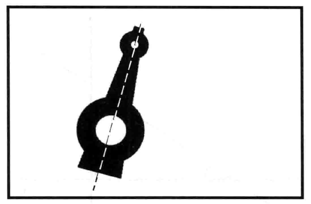
如果我们想要知道二值图物体表示的朝向，则需要用到转动惯量的概念。如果找到了使得物体转动惯量最小的轴，那么这个轴向就是物体的朝向。
在当前图像为二维的情况下，转动惯量是物体针对某条直线，将物体上的每个点到直线距离的平方按照密度计算积分，即得到了图像关于该轴向的转动惯量值。
我们的任务是为给定的二值图物体找到使得其转动惯量最小的直线。
转动惯量计算方法：

$$
E=\iint_{I} r^{2} b(x, y) d x d y \tag{4} \label{4}
$$

其中 $r$ 表示二值图上的点到直线的距离，虽然还没有这条直线

直线建模

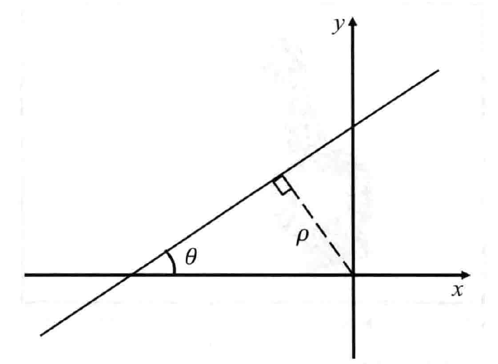
为我们的目标直线建模，取2个参数
- 原点到直线的距离 $\rho$
- 直线和 $x$ 轴之间（沿逆时针方向）的夹角 $\theta$
这种建模方式有一些方便之处：
- 当坐标系平移或旋转时，这两个参数的变化是连续的
- 当直线平行（或近似平行）于某个坐标轴时，用这两个参数来表示直线也不会产生问题（相比于：使用斜率和截距来表示直线的情况）
使用这两个参数，可以将直线方程写为如下形式：

$$
x \sin \theta-y \cos \theta+\rho=0 \tag{5} \label{5}
$$

在直线上，距离原点最近的点$ (-\rho \sin \theta,+\rho \cos \theta) $，通过这个点，沿着夹角 $\theta$ 运动任意距离$s$ 的点仍在直线上，因此可以将直线上任意一点$(x_0,y_0)$表示为：

$$ \begin{array} { l } { x _ {0 } = - \rho \sin \theta + s \cos \theta } \\ { y _ {0} = + \rho \cos \theta + s \sin \theta } \end{array} \tag{6} \label{6} $$

最短距离

回到我们的二值图，在给定直线方程的情况下，二值图上一点$(x,y)$，直线上距离其最近的点$(x_0,y_0)$，二者距离显然可以表示为：

$$ r^{2}=\left(x-x_{0}\right)^{2}+\left(y-y_{0}\right)^{2} \tag{7} \label{7} $$

将直线上点公式$\eqref{6}$代入，得到：

$$ r^{2}=x^{2}+y^{2}+\rho^{2}+2 \rho(x \sin \theta-y \cos \theta)-2 s(x \cos \theta+y \sin \theta)+s^{2} \tag{8} \label{8} $$

对于每个点，我们都需要解$\eqref{8}$这样的优化方程
即给定了$x,y,\rho,\theta$，求解使得$r$最小的s$,我们在$$\eqref{8}$中对$s$求导，可得：

$$
s=x \cos \theta+y \sin \theta \tag{9} \label{9}
$$

将$\eqref{9}$带入$\eqref{6}$，二值图上$(x,y)$到直线上距离最近的点$(x_0,y_0)$可得到关系为：

$$ x-x_{0}=+\sin \theta(x \sin \theta-y \cos \theta+\rho) \\ y-y_{0}=-\cos \theta(x \sin \theta-y \cos \theta+\rho) \tag{10} \label{10} $$

将$\eqref{10}$带入 $\eqref{7}$可得：

$$
r^{2}=(x \sin \theta-y \cos \theta+\rho)^{2} \tag{11} \label{11}
$$

此处可以看到，将某点$(x,y)$带入$\eqref{5}$，得到值的绝对值即为该点到直线的垂线（最短）距离。

二阶矩轴向通过质心

我们已经得到了二值图上一点到任意直线的距离计算方法，将$\eqref{11}$带入$\eqref{4}$，得到：

$$ \begin{aligned} E&=\iint_{I}(x \sin \theta-y \cos \theta+\rho)^{2} b(x, y) d x d y \\ &=\iint_{I}[{(x\sin \theta - y\cos \theta )^2} + {\rho ^2} + 2\rho (x\sin \theta - y\cos \theta )]b(x,y)dxdy\\ &=[{(x\sin \theta - y\cos \theta )^2} + {\rho ^2}]\iint_{I}b(x,y)dxdy + 2\rho \sin \theta \iint_{I}xb(x,y)dxdy - 2\rho \cos \theta \iint_{I}{yb(x,y)dxdy} \end{aligned} \tag{12} $$

对$\rho$求导，并令倒数为0，得到：

$$
(\bar{x} \sin \theta-\bar{y} \cos \theta+\rho) A=0\tag{13}
$$

其中，A是区域面积，而是区域质心。因此，我们得到了结论：

$$
最小二阶矩所对应的轴一定经过区域重心！
$$

确定轴向倾角

我们已经确定该轴经过一个确定的点$ (\bar{x}, \bar{y}) $了，仅需要再确定直线倾角即可。

将二值图平移到原点与质心重合的位置，那么我们要求得的就是一条穿过原点的直接倾角
也就是直接去除 $\rho$ 参数的影响
转动惯量计算方式如下：

$$
E=\iint_{I}(x’ \sin \theta-y’ \cos \theta)^{2} b(x’, y’) d x’ d y’ \tag{14}
$$

其中，我们定义平移后的二值图$I’$上点的坐标为$ ({x’}, {y’}) $。

可以表示为：

$$ \begin{array}{l} E=a \sin ^{2} \theta-b \sin \theta \cos \theta+c \cos ^{2} \theta \\ 其中： a=\iint_{I^{\prime}}\left(x^{\prime}\right)^{2} b\left(x^{\prime}, y^{\prime}\right) d x^{\prime} d y^{\prime} \\ b=2 \iint_{I^{\prime}}\left(x^{\prime} y^{\prime}\right) b\left(x^{\prime}, y^{\prime}\right) d x^{\prime} d y^{\prime} \\ c=\iint_{I^{\prime}}\left(y^{\prime}\right)^{2} b\left(x^{\prime}, y^{\prime}\right) d x^{\prime} d y^{\prime} \\ \end{array} \tag{15} \label{15} $$

即：

$$
E=\frac{1}{2}(a+c)-\frac{1}{2}(a-c) \cos 2 \theta-\frac{1}{2} b \sin 2 \theta \tag{16}
$$

上式对$\theta$求导，并令求导结果等于零
假设$a≠c$，我们可以得到：

$$
\tan 2 \theta=\frac{b}{a-c} \tag{17} \label{17}
$$

因此除非出现$ b=0 $ 并且 $ a=c $ 的情况, 否则, 我们最终可以得到：

$$ \begin{array}{l} \sin 2 \theta=\pm \frac{b}{\sqrt{b^{2}+(a-c)^{2}}} \quad \\ \cos 2 \theta=\pm \frac{a-c}{\sqrt{b^{2}+(a-c)^{2}}} \end{array} \tag{18} $$

至此我们已经求出了使得该二值图转动惯量最小和最大的两个轴
$E$ 的的最小值和最大值的比值，给出了一些关于物体有“多么圆”的信息。对于直线，这个比值是0对于圆，这个比值是1。

拉格朗日

从式$\eqref{15}$开始，事实上我们要解的就是一个带约束的优化方程组，可以使用拉格朗日乘数法求解：

$$ \begin{array}{l} E = a{x^2} - bxy + c{y^2}\\ s.t.{x^2} + {y^2}-1 = 0 \end{array} \tag{19} \label{19} $$

将$E$设为$f(x,y)$，约束条件设为$g(x,y)=0$，构建拉格朗日方程：

$$
L(x,y) = a{x^2} - bxy + c{y^2} + \lambda ({x^2} + {y^2}-1) \tag{20}
$$

构造拉格朗日方程组：

$$ \left\{ \begin{array}{l} \frac{{\partial f}}{{\partial x}} + \lambda \frac{{\partial g}}{{\partial x}} = 0\\ \frac{{\partial f}}{{\partial y}} + \lambda \frac{{\partial g}}{{\partial y}} = 0\\ g(x,y) = 0 \end{array} \right. \to \left\{ \begin{array}{l} 2ax - by + 2\lambda x = 0\\ 2{\rm{cy}} - bx + 2\lambda y = 0\\ {x^2} + {y^2} = 1 \end{array} \right. \tag{21} $$

重新令 $x = sin\theta, y=cos \theta$ 可得：

$$ \begin{array}{l} 2a - b\frac{1}{{\tan \theta }} = 2c - b\tan \theta \\ b(ta{n^2}\theta - 1) + 2(a - c)tan\theta = 0\\ \frac{b}{{a - c}} = \frac{{2\tan \theta }}{{{{\tan }^2}\theta - 1}} = \tan 2\theta \end{array} \tag{22} $$

即推出$\eqref{17}$相同结论。

特征向量

可以将$\eqref{19}$看作是一个二次型优化问题，原带约束的方程可以写成：

$$ \begin{array}{*{20}{l}} {E = {{\bf{s}}^T}{\bf{As}}}\\ {s.t.1-{{\bf{s}}^T}{\bf{Is}} = 0} \end{array} \tag{23} $$

其中: ${\bf{s}} = \left( \begin{array}{l} x\\ y \end{array} \right)$，${\bf{A}} = \left( \begin{array}{l} \begin{array}{*{20}{c}} a&{\frac{b}{2}} \end{array}\\ \begin{array}{*{20}{c}} {\frac{b}{2}}&c \end{array} \end{array} \right)$，$\bf{I}$为二阶单位阵
那么拉格朗日方程可以写成：

$$ {L = {{\bf{s}}^T}{\bf{As}} - \lambda(1- {{\bf{s}}^T}{\bf{Is}}}) \tag{24} $$

$L$对$\bf{s}$的偏导数为0：

$$ \begin{array}{l} \frac{{\partial L}}{{\partial {\bf{s}}}} = 2{\bf{As}} - 2\lambda {\bf{Is}} = 0\\ {\bf{As}} = \lambda {\bf{s}} \end{array} \tag{25} \label{25} $$

而式$\eqref{25}$就是在寻找矩阵$\bf{A}$的特征向量和特征值。
也就是说，对于给定的二值图，求解其对应的$a,b,c$，构造出矩阵$\bf{A}$，求解$\bf{A}$的特征向量即是寻找最大、最小转动惯量的方向。
二者大小的比值也类似于特征值的比值，也就是矩阵的条件数。

参考示例

示例图像：

示例程序

import math
import cv2

import numpy as np

import matplotlib.pyplot as plt
from numpy.lib.function_base import iterable


def vvd_round(num):
    if iterable(num):
        return np.round(np.array(num)).astype('int32').tolist()
    return int(round(num))


def show_image(image):
    plt.imshow(image.astype('uint8'))
    plt.show()
    pass


def gravity_center(mask):
    Ys, Xs = mask.nonzero()
    A = (mask > 0).sum()
    C_X = (Xs).sum() / A
    C_Y = (Ys).sum() / A
    return C_X, C_Y


def load_gray_image(image_path):
    image = cv2.imread(image_path)
    image = cv2.cvtColor(image, cv2.COLOR_BGR2GRAY)
    image = (image == 0).astype('uint8') * 255
    return image


def moment_of_inertia(mask, center):
    temp_image = mask.copy().astype('uint8') * 128

    C_X, C_Y = center

    Ys, Xs = mask.nonzero()

    Ys = (Ys - C_Y) / 100
    Xs = (Xs - C_X) / 100

    a = (Xs * Xs).sum()
    b = 2 * (Xs * Ys).sum()
    c = (Ys * Ys).sum()

    if b == 0:
        theta = 0
    elif a == c:
        theta = - np.pi * 0.5 * 0.5
    else:
        theta = - math.atan(b / (a - c)) / 2

    point_1 = vvd_round([C_X + math.cos(theta) * 200, C_Y - math.sin(theta) * 200])
    point_2 = vvd_round([C_X - math.cos(theta) * 200, C_Y + math.sin(theta) * 200])

    temp_image = cv2.line(temp_image.astype('uint8'), point_1, point_2, 255, 2)

    point_1 = vvd_round([C_X + math.cos(theta + 0.5 * np.pi) * 200, C_Y - math.sin(theta + 0.5 * np.pi) * 200])
    point_2 = vvd_round([C_X - math.cos(theta + 0.5 * np.pi) * 200, C_Y + math.sin(theta + 0.5 * np.pi) * 200])

    temp_image = cv2.line(temp_image.astype('uint8'), point_1, point_2, 200, 2)

    theta_1 = theta
    theta_2 = theta + 0.5 * np.pi

    E_1 =(math.sin(theta_1)) ** 2 * a - b * math.sin(theta_1) * math.cos(theta_1) + c * (math.cos(theta_1)) ** 2
    E_2 =(math.sin(theta_2)) ** 2 * a - b * math.sin(theta_2) * math.cos(theta_2) + c * (math.cos(theta_2)) ** 2

    return temp_image, min(E_2, E_1) / max(E_2, E_1, 1)


if __name__ == '__main__':
    image_path = 'test.png'
    image = load_gray_image(image_path)
    center = gravity_center(image)
    temp_image, rate = moment_of_inertia(image, center)
    show_image(temp_image)
    pass